Introduction

Plants are increasingly being recognized for their medicinal value and are being consumed and processed specifically for the prevention and treatment of various diseases (Mocan et al., 2016; Li and Weng, 2017). Consequently, the market for plant-based raw materials intended to be used for making supplements and medicine is growing globally. Particularly, there is an increasing interest in berries, which can be added to beverages or processed as powders, because they contain high amounts of bioactive compounds (Llorent-Martínez et al., 2013).

Lycium barbarum, L. chinense, Cornus officinalis, and Schisandra chinensis have been used historically as food and medicine in East Asia (Llorent-Martínez et al., 2013; Li and Weng, 2017). L. barbarum and L. chinense are deciduous shrubs and bear bright orange-red oval berries measuring 1 to 2 cm long, with the corresponding common names of goji berry and wolfberry (Donno et al., 2015), known as “gugija” in Korean. These berries have great benefits for eye health because it contains bioactive substances such as zeaxanthin and lutein (Chien et al., 2018; Skenderidis et al., 2022; Teixeira et al., 2023). C. officinalis has red berries that are oblong and 1.5 to 2 cm long, known as “sansuyu” in Korean. This plant has pharmacological effects associated with digestive improvements and the enhancement of liver and kidney functions (Gao et al., 2021; Fan et al., 2022). S. chinensis produces red, spherical berries about 1 cm in diameter, known as “omija” in Korean. The consumption of S. chinensis berries has been reported to enhance the immune response (Li et al., 2018; Kortesoja et al., 2019).

Berries of medicinal plants, offered as over-the-counter remedies or herbal supplements, are utilized by many patients for self-prescribed therapeutic practices in their daily lives (Chen et al., 2010). However, interactions between various foods and medicinal plants can lead to unwanted side effects (Karimpour-Reihan et al., 2018). For example, cases in which patients with chronic cardiovascular disease experienced toxicity due to the inhibition of the CYP2D6 enzyme involved in flecainide metabolism after consuming L. barbarum as a supplement have been reported (Guzmán et al., 2021). Moreover, due to the similarities in physical traits such as the size, shape, and color, many medicinal plants and their fruits can be difficult to distinguish visually, leading to misidentification (Rajani and Veena, 2022).

Therefore, to identify medicinal plants accurately, recent research has focused on exploring methods for differentiating the color and shape more accurately (Fu et al., 2011; Karki et al., 2024). Plants with similar colors, textures, and geometric features have been accurately distinguished through imaging by means of optical microscopy, followed by feature extraction and the utilization of a decision tree model with accuracy rates exceeding 95% (Keivani et al., 2020). Wang et al. (1999) employed optical radiation measurements to differentiate rice grains by color. They measured the reflectance spectra log (1/R) in the 400 nm–2000 nm wavelength, achieving accuracy rates up to 98.5% by utilizing partial least squares (PLS) regression. However, the techniques mentioned are destructive and time-consuming (Ariana and Lu, 2010).

To eliminate time-consuming sample preparation and measurement processes and destructive testing, hyperspectral technology can be applied to medicinal plant identification (Liu et al., 2022). Hyperspectral imaging systems disperse incident light to acquire very large amounts of spectral information corresponding to each pixel in an image. Hyperspectral imaging enables high-resolution analyses of small areas and is particularly effective if used to analyze and monitor colors in specific parts of objects (Chlebda et al., 2017). Consequently, selecting an appropriate machine learning model is crucial for interpreting high-dimensional hyperspectral data containing a large amount of spectral information (Makantasis et al., 2018; Baek et al., 2023).

Few studies have used hyperspectral imaging to classify plants with similar colors, and an identification accuracy rate of 98.1% was achieved in one study that applied machine learning to hyperspectral images (Ruett et al., 2022). Another study used hyperspectral imaging to differentiate various plants with different colors (Salve et al., 2022). However, research on identifying the fruits of medicinal plants with similar colors through hyperspectral imaging is lacking.

In this study, a classification framework applying machine learning techniques to hyperspectral images of representative medicinal plants producing berries with similar colors and sizes (C. officinalis, L. chinense, L. barbarum, and S. chinensis) is developed and evaluated. Four supervised learning models were evaluated: logistic regression (LR), K-nearest neighbor (KNN), decision tree (DT), and random forest (RF) models. Considering the challenges posed by the high-dimensional and redundant data of hyperspectral images, the selected models offer complementary strengths. LR provides simplicity and efficiency in high-dimensional spaces, KNN captures local patterns, the DT model handles non-linear relationships and feature selection, and RF, given its ensemble characteristic, enhances robustness and copes with dimensionality effectively. The novel identification technology using hyperspectral images can be applied at the commercial distribution stage and thus contribute to controlling the product quality and ensuring the authenticity of medicinal fruits.

Materials and Methods

Sample collection

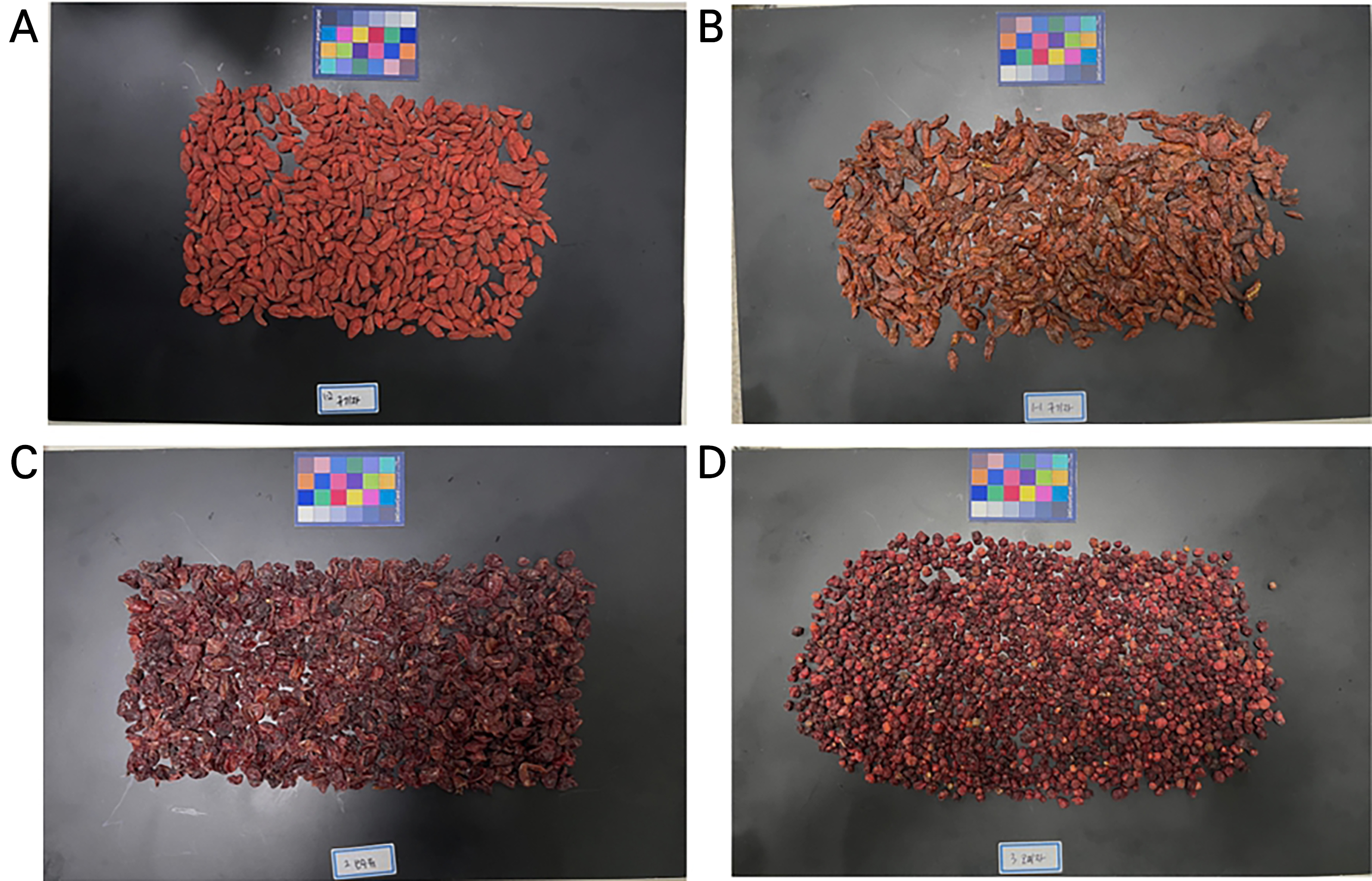
Dried fruits of four different medicinal plants, C. officinalis, L. chinense Miller, L. barbarum Linné, and S. chinensis, were purchased from local markets in Gangneung, Korea (Fig. 1). The red fruits of these four species are all oval-shaped with a diameter of 1–2 cm. The species were identified and verified by experts. The weights of each sample used in the experiment are as follows: C. officinalis 155 g, L. chinense 146 g, L. barbarum 179 g, and S. chinensis 160 g.

Fig. 1.

Photographs of the collected samples: ((A) C. officinalis, (B) L. chinense, (C) L. barbarum, (D) S. chinensis).

Hyperspectral imaging system

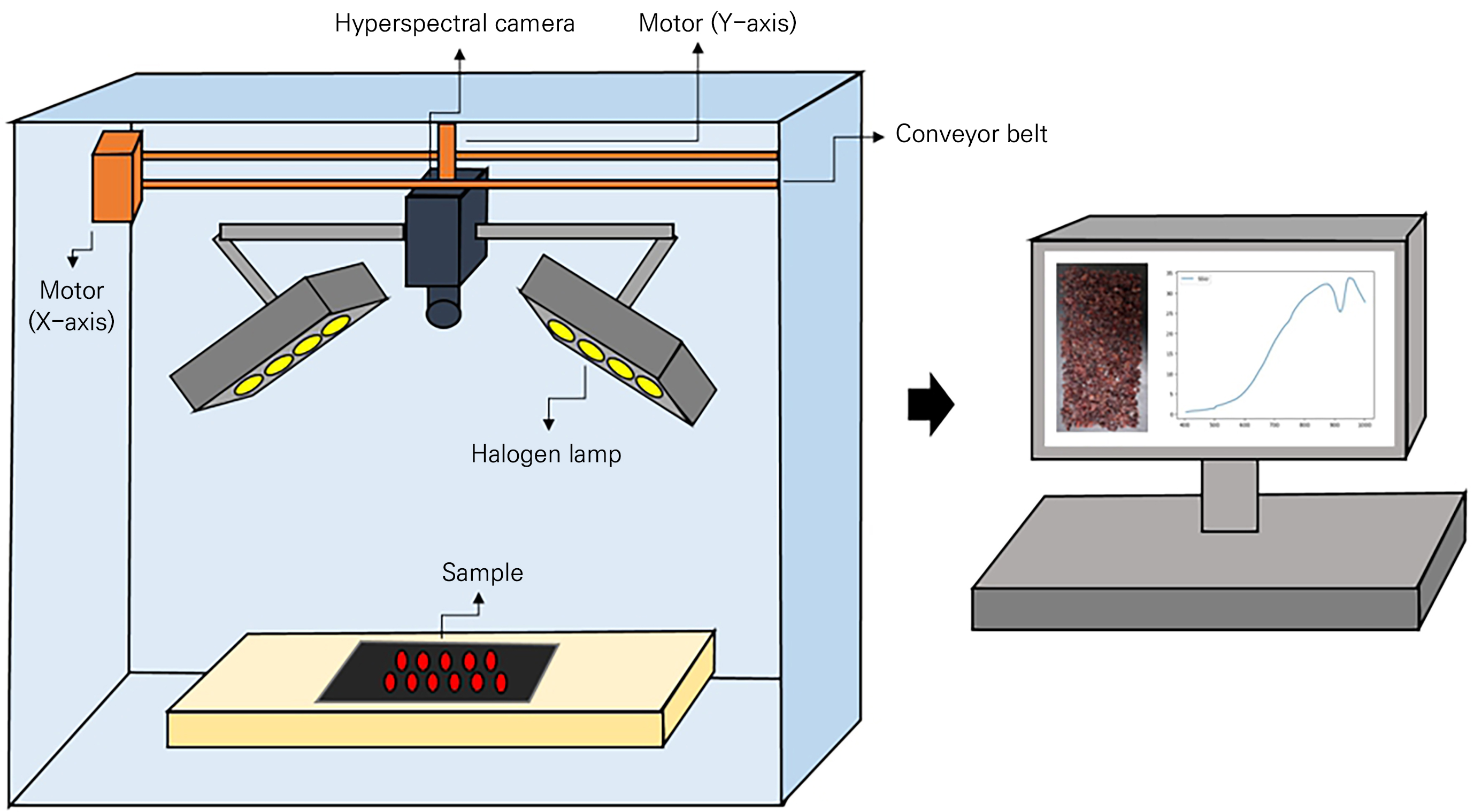
Hyperspectral images were captured using a MicroHSI 410 SHARK (Corning Inc., Corning, NY, USA) camera with eight 20 W halogen lamps mounted on the side of the camera (four on each side) to illuminate the sample (Fig. 2). The camera setup can be moved along the X- and Y-axes using a conveyor belt and a motor, and the speed can be adjusted while capturing images in a line-scan manner. The images were obtained with 150 wavelength bands within the 404.52–1000.88 nm range at a rate of 100 mm·s^-1 on the X-axis. Each sample was placed in the central part, where the light distribution was uniform, on a non-reflective black panel.

Fig. 2.

Schematic of the hyperspectral measurement setup.

Dataset extraction

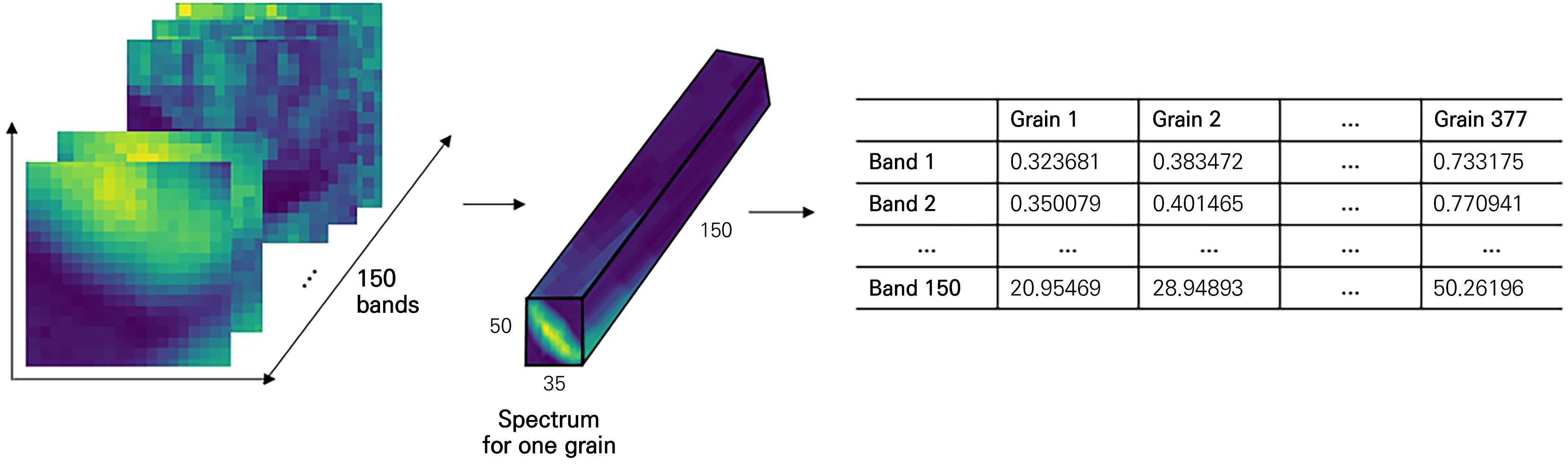
To generate training data for the classification model from the raw data of the hyperspectral images acquired as described above, we followed the process depicted in Fig. 3. First, for each hyperspectral image, each sample fruit was individually selected as a region of interest (ROI). Given the differing size and shape of each berry, the ROI size was set differently (Fig. 3B and 3C). The data shape of one ROI was assigned as 48×32×150 for C. officinalis, 50×35×150 for L. chinense, 50×28×150 for L. barbarum, and 28×18×150 for S. chinensis. As a result, there were correspondingly 327, 377, 424, and 1,070 multiple ROI counts.

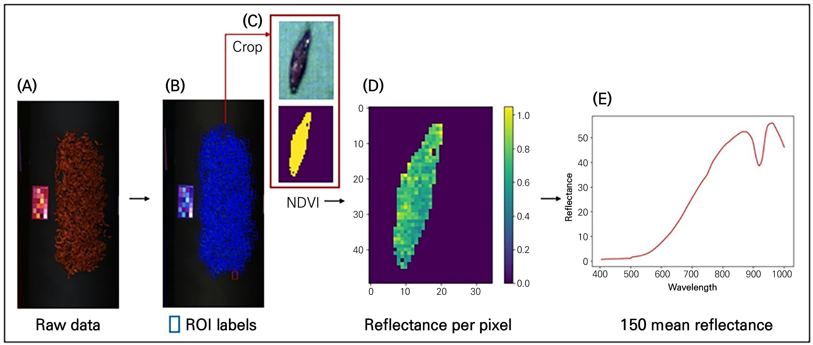
Fig. 3.

Process of extracting training data: ((A) Raw data captured with a hyperspectral camera, (B) selection of regions of interest (ROIs) for each berry sample, (C) separation of background and sample using a single berry crop and the application of NDVI, (D) reflectance for each pixel of the sample berry, and (E) average reflectance values across 150 spectral bands for a single sample berry).

Second, a thresholding technique using the normalized difference vegetation index (NDVI) was applied for background removal (Fig. 3C and 3D). NDVI is generally used for quantifying vegetation and is calculated from spectral data at the near-infrared (NIR) and red light (RED) bands (Hashim et al., 2019; Agilandeeswari et al., 2022):

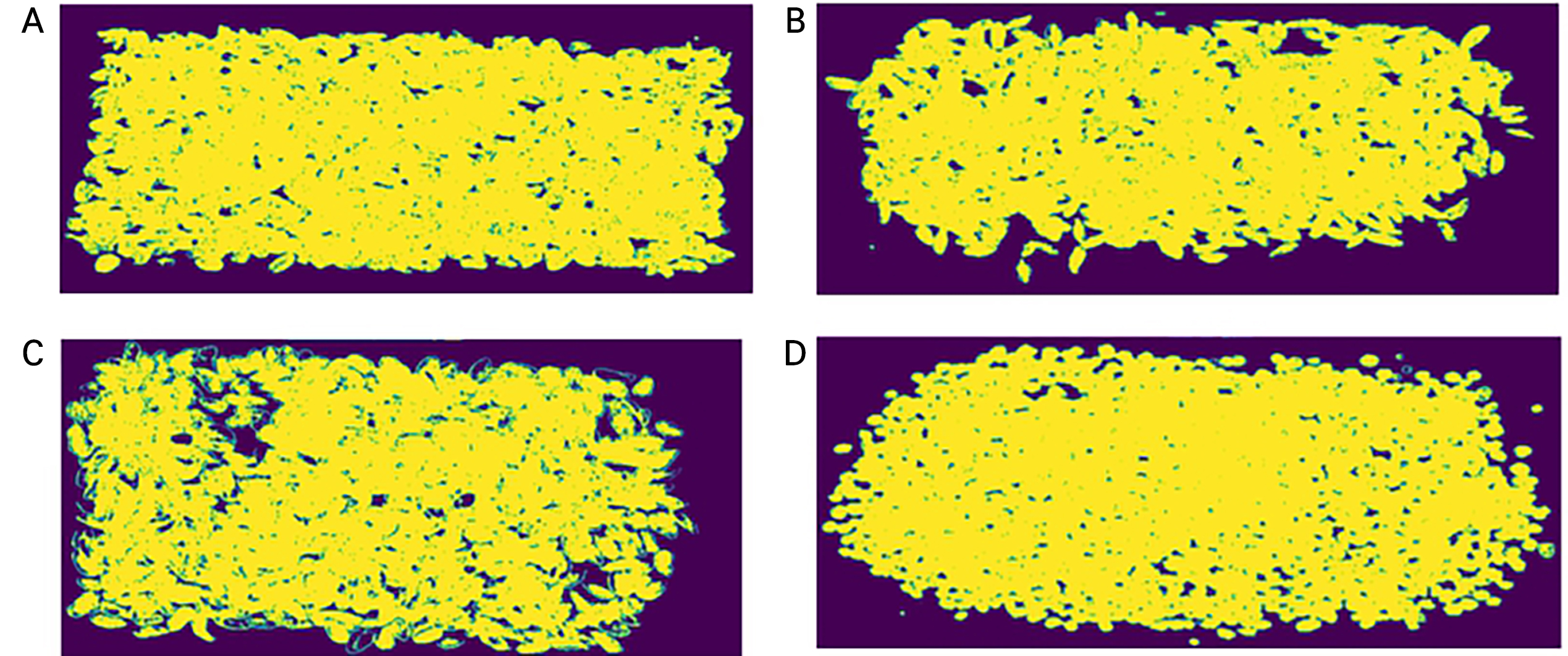
In this study, NDVI values for each pixel were calculated from 812.76 and 652.67 nm as the NIR and RED bands, respectively. An NDVI-based segmentation mask was created with a threshold value of 0.3 (Fig. 4). The threshold was determined as the value that most strengthens the contrast between dried berries and the background. After background removal, the reflectance values were compared with the raw data to confirm the segmentation results (Fig. 3D). Despite the fact that this study did not target leaves, NDVI was used because it can effectively separate background materials as well as non-plant contaminants regardless of the plant species.

Fig. 4.

Removing the background using NDVI: ((A) C. officinalis, (B) L. chinense, (C) L. barbarum, (D) S. chinensis).

Finally, the average reflectance per cropped berry for each sample was extracted. Some ROIs were calculated while including a single intact berry and a portion of an adjacent berry. Files in the npy format saved per sample were formed as two-dimensional data with one average data instance per band (Fig. 5). This process of generating the training data was conducted in the Python 3.8 environment using the numpy, pandas, and matplotlib libraries.

Fig. 5.

Process of converting 3D data to 2D data and then extracting the mean reflectance for each band (Lycium chinense).

Machine learning model for classification

The generated training data were applied to four artificial intelligence models: LR, KNN, DT, and RF. These models were utilized to classify the training data into four classes: C. officinalis, L. chinense, L. barbarum, and S. chinensis.

LR is a generalized linear model with a standard link function (Golpour et al., 2020). It is widely used as a data processing method for analyzing and estimating relationships among various data in both binary classification and predictive aspects. This model predicts whether data belong to a specific category, assigning a continuous probability rate between 0 and 1 (Zou et al., 2019). The probability of the event of interest (pi) occurring is determined as follows:

The probability of occurrence is a function of the explanatory variable vector (x_i), a set of common underlying weights (𝜔), and a constant (b) shared across all observations. The subscript (i) represents one unique observation from a total of N observations (Robles-Velasco et al., 2020).

KNN is one of the most essential and effective algorithms for data classification. It is a method used to classify objects based on the closest training examples in feature space (Boateng et al., 2020; Bansal et al., 2022). Unlike typical machine learning models, it does not require a separate training phase to construct a predefined model (Wang et al., 2023). Instead, KNN relies on the entire training dataset during the classification phase to identify the nearest neighbors for a given sample. Therefore, it can classify new data based on the arrangement and similarity of its nearest neighbors, resulting in a straightforward and accurate prediction (Rajaguru and S R, 2019). The KNN algorithm uses the Euclidean distance measurement method to find the nearest neighbors. The distance d(x,y) between two points x and y is calculated as follows:

where N is the number of features, x = {x₁, x₂, x₃, ..., x_N}, and y = {y₁, y₂, y₃, ..., y_N} (Boateng et al., 2020; Shabani et al., 2020; Wang et al., 2023).

DT is a machine learning model that extracts data based on specific criteria from feature-based samples (Rajaguru and S R, 2019; Zhou et al., 2021). Additionally, it has relatively few parameters to estimate because it divides the variable space into two spaces at each branching step. Furthermore, the DT algorithm proceeds with learning in a way that minimizes uncertainty. Uncertainty refers to how different data are mixed within a category. Degrees of Uncertainty or disorder are quantified by a measure called entropy. When disorder is minimal, meaning there is only one data point in a category, the entropy is 0. In other words, by gaining information, the DT is constructed, and the data are split using the maximum entropy reduction attribute (Li et al., 2019).

RF is a machine learning approach that uses the DT learning algorithm. It is widely used for developing predictive models (Shabani et al., 2020). It is an ensemble learning approach, where the same problem is divided into many small sets of data through resampling to create a diverse dataset, followed by training. The idea is to combine multiple learning models to improve the accuracy. This allows for a reduced number of required variables, thus reducing the burden of data collection and improving the efficiency (Sheykhmousa et al., 2020). To construct each individual tree within the RF model, variables are randomly selected from the training set, and the best splitting criteria are explored within the subset of randomly chosen variables (Speiser et al., 2019). This randomness leads to greater diversity among the trees and reduces unrelated trees, thereby enhancing the overall performance. As a result, to make predictions for a given set of test observations, the individual trees predict classes, and the final prediction is made in classification problems by majority voting, where the most frequently predicted class is chosen (Han et al., 2021).

Multi-class classification to classify four medicinal plants using the models described earlier was conducted. In this process, the scikit-learn library in the Python environment was utilized, and multi-class classification was addressed by employing the One-vs-Rest strategy. One-vs-Rest involves training one binary classifier for each class, as some classifiers that perform well in binary classification may not easily extend to multi-class classification problems (Faris et al., 2020).

The ratio of the training data to the test data was divided into an 8:2 split, and a K-fold cross-validation process was conducted by dividing the training dataset into ten subsets and sequentially cross-validating them as test data. This was done to address potential issues that may arise when working with limited data, allowing for the repetitive evaluation of the model performance on the training set (Wong and Yeh, 2019).

Evaluation of machine learning models

Performance metrics were used to evaluate whether the classification of samples using the previously described models was appropriate (Adikari et al., 2021). Improving the predictive performance of artificial intelligence models is a crucial process. In this study, we utilized four classification model performance evaluation metrics: a confusion matrix, accuracy, the F1 score, and the ROC curve.

The confusion matrix is a visual evaluation tool for assessing the performance of a classification model in machine learning (Heydarian et al., 2022). It classifies items by comparing actual labels with the model's predicted results. In this case, columns represent the results of predicted classes, and rows represent the results of actual classes. Given that four classes are used for classification models, a total of 16 outcomes are produced. This allows the definition of a series of algorithm performance metrics (Theissler et al., 2022).

Accuracy values quantify the proportion of correct predictions out of all predictions. A higher accuracy value indicates higher prediction accuracy, aiding in the distinction of each class. Accuracy is relatively straightforward to compute and has low complexity. Additionally, it is readily applicable to both multi-class and multi-label problems (Bochkovskiy et al., 2020).

The F1 score measures the harmonic mean between recall and precision. Recall represents the number of truly positive data instances that the model correctly identifies as positive, while precision represents the ratio of instances the model correctly identified as positive to the total instances it classified as positive (Salman et al., 2020). There are three types of F1 scores, and their differences lie in how they calculate the average. Firstly, the macro-average is simply the average F1 score across labels. The weighted average assigns weights proportional to the number of labels and then averages the F1 scores, while the micro-average computes the F1 score by considering the entire sample as a whole (Zeng et al., 2023). In this study, to mitigate the impact of varying training sample sizes on the F1 scores, the macro-average method was employed.

The ROC curve plots sensitivity against 1-specificity and graphically shows how different levels of sensitivity affect specificity. It allows for a quick understanding of the utility of an algorithm and can be used to evaluate the level of classification (Handelman et al., 2019).

Results and Discussion

Spectral analysis results in hyperspectral data

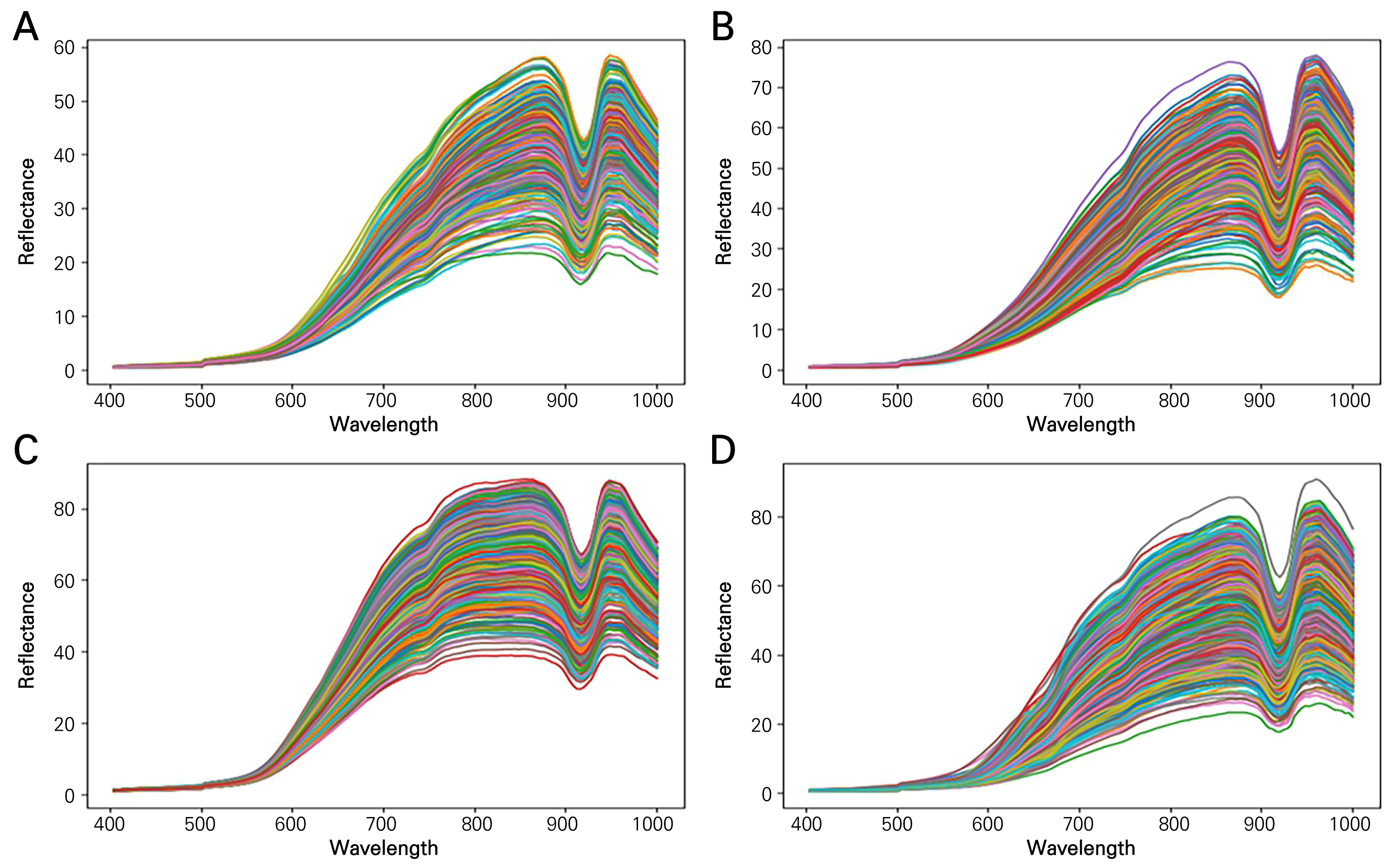
After obtaining the average reflectance within each sample ROI (Fig. 6), the maximum and minimum reflectance values were examined. In the order of C. officinalis, L. chinense, L. barbarum, and S. chinensis, the maximum values were 58.3%, 77.7%, 86.9%, and 90.7%, respectively. The corresponding minimum values were 0.06%, 0.09%, 0.15%, and 0.08%. The overall shape was similar across all samples, but a sharp decrease was observed around 900 nm. This can be attributed to the sensitivity limitations of the hyperspectral camera, as indicated in the camera specifications. Similar decreases in reflectance around 900 nm have been observed in other studies that used the same camera (Choi et al., 2022). This suggests that the type of equipment used can impact the results.

Fig. 6.

Average reflectance of 150 spectral bands per cropped specimen unit: ((A) C. officinalis, (B) L. chinense, (C) L. barbarum, (D) S. chinensis).

Model evaluation based on classification model evaluation metrics

Accuracy/F1 score

The accuracy and F1 scores for the classification models are summarized in Table 1. The accuracy values for the test data were all above 90%, indicating a high probability of correct classification. Likewise, the F1 scores were all above 0.9, approaching 1, demonstrating that most of the models exhibited effective performance. Notably, the values were consistently close to 1, indicating that overfitting did not occur during the data splitting process between the training and test datasets. Furthermore, in terms of the classification results for the test data, the LR model had the highest accuracy and F1 scores, both at 0.998, followed by RF, DT, and KNN in descending order of performance.

The experiments with the training and test data were validated using the K-fold cross-validation method, and Table 1 presents the averaged accuracy and F1 score results after ten rounds of performance evaluations. All four models consistently achieved high values around 0.9, demonstrating the effectiveness of the models in correctly classifying the samples. Furthermore, all datasets were used for training, resulting in improved accuracy and F1 score outcomes. This prevented underfitting due to data scarcity and reduced bias in the evaluation data. In this study, the processing times of the LR, KNN, DT, and RF models were approximately 2.1, 0.3, 2.2, and 12 seconds, respectively, during training, testing, and cross-validation. The processing time of a model is an important factor to consider with regard to computational efficiency, especially for field applications such as software or device development. In this study, where there was a significant difference in the number of data samples used, this approach proved effective in achieving more generalized results and contributed to the more effective application of the data to the models.

Confusion matrix

The confusion matrices for the four classification models are presented in Fig. 7. Overall, all machine learning models used here showed appropriate classification with high probabilities. In particular, the LR model exhibits the best results, correctly classifying all samples. LR was expected to perform efficiently in hyperspectral image classification due to several specific features. Hyperspectral images are characterized by high-dimensional data and a large number of spectral bands, making feature extraction and classification challenging (Ham et al., 2005; Li et al., 2009; Qian et al., 2012; Kishore and Kulkarni, 2016).

Fig. 7.

Confusion matrix for each classification model: ((A) Logistic Regression (LR), (B) K-Nearest Neighbor (KNN), (C) Decision Tree (DT), (D) Random Forest (RF)).

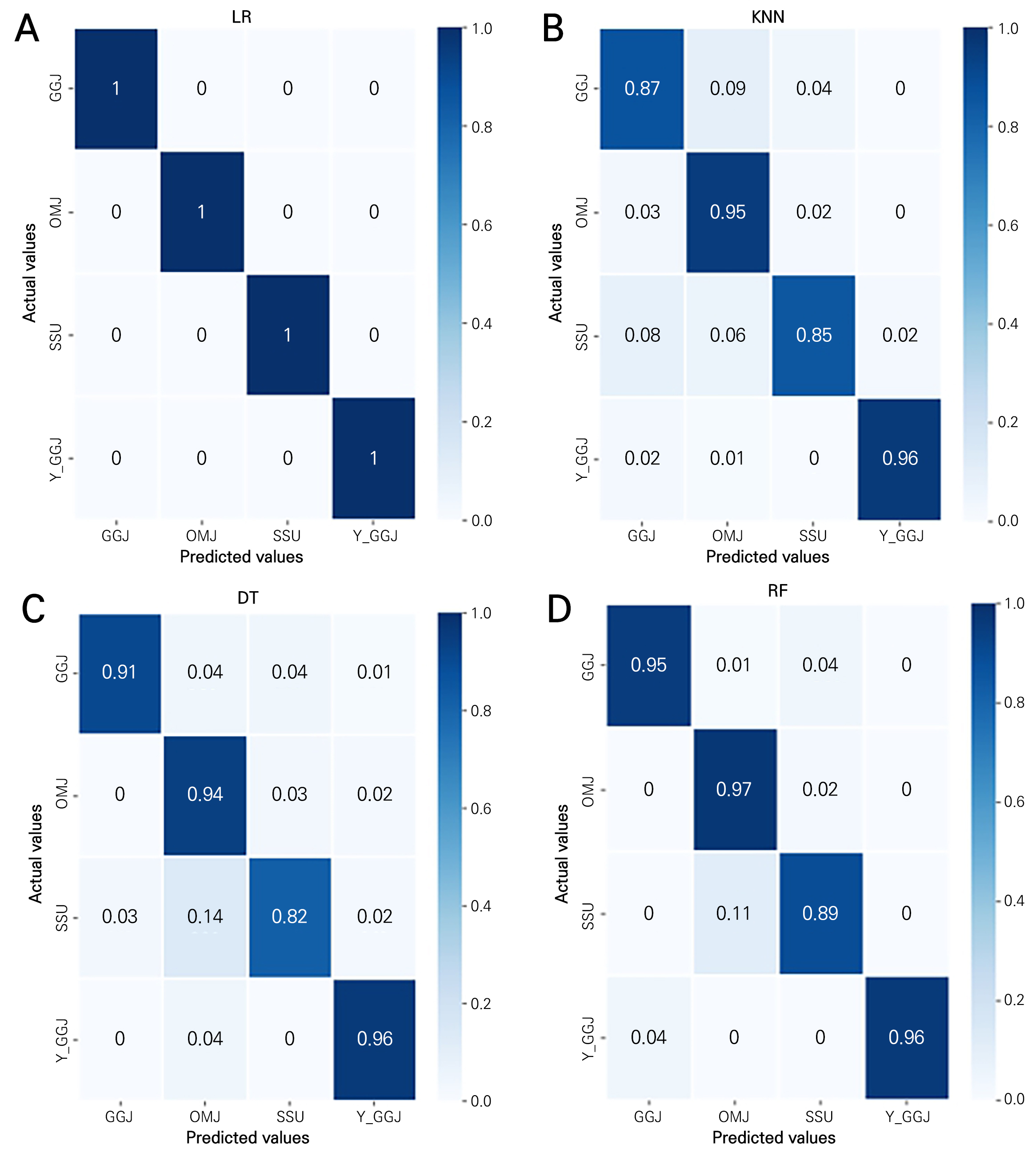
The LR model seeks linear decision boundaries to classify data into multiple categories. Linear decision boundaries help classify data in diverse and intuitive ways (Li et al., 2009; Golpour et al., 2020). Consequently, the LR model does not implement a complex classification process, similar to the KNN and DT models. This simplicity is one of its advantages. Therefore, the combination of hyperspectral data and the LR model provides an effective approach for data classification, allowing for straightforward modeling. As a result, this combination helps process extensive hyperspectral data and obtains accurate results (Kishore and Kulkarni, 2016).

LR also has the ability to learn class distributions (Shah et al., 2020). This feature is highly valued in the context of hyperspectral data. LR learns the distribution for each class and estimates the probability of each data point belonging to a specific class (Gautam and Nadda, 2022; Ye et al., 2022). This capability turns it into a powerful tool for modeling relationships among multiple classes. By utilizing this ability, not only can data be effectively classified, but also interactions and dependencies among classes can be taken into account. On the other hand, classification models such as KNN or DT do not directly learn class distributions but classify data based on factors such as neighboring points or splitting rules. This makes it challenging to consider relationships among classes or achieve proper classification in datasets with class imbalances.

In previous research related to actual hyperspectral image classification models, LR demonstrated an accuracy rate close to 100%, with a true positive rate (TPR) near 1 and a false positive rate (FPR) close to 0, making the ROC curve results highly satisfactory (Feng et al., 2019). Therefore, it is confirmed that LR exhibits outstanding capabilities for effective classification.

ROC curve

The classification models were evaluated using ROC curves and the corresponding AUC values (Fig. 8). It can be observed that, in general, the AUC values for all ROC curves are approximately 0.9, indicating that classification was carried out appropriately. For the LR model, all AUC values are close to 1, confirming that all samples were correctly classified. KNN and RF also achieved AUC values of 0.98 or higher, demonstrating effective classification. However, among the four models, DT has the lowest AUC value. This can be explained in comparison to RF, as both models utilize a tree-based structure for data analysis and prediction. However, RF combines multiple DTs to reduce overfitting tendencies, increase model diversity, and improve generalization performance.

Fig. 8.

ROC curves and AUC values for each classification model: ((A) Logistic Regression (LR), (B) K-Nearest Neighbor (KNN), (C) Decision Tree (DT), (D) Random Forest (RF)).

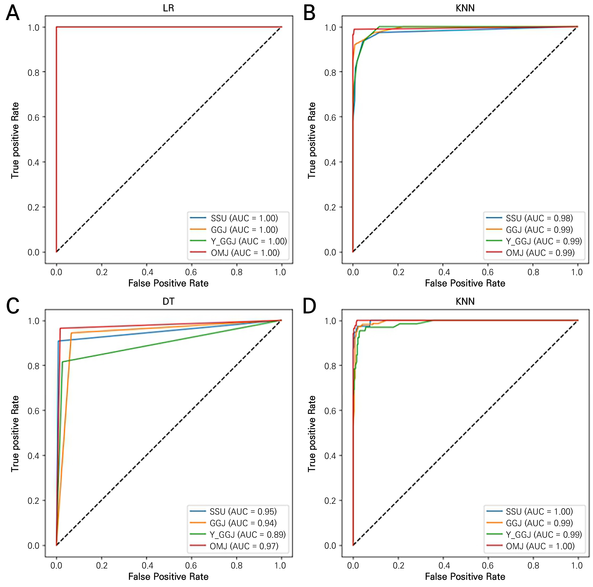
In previous studies related to hyperspectral image classification using both models, the RF model demonstrated results with AUC values very close to 1. However, for classification using DT, the AUC values were between 0.6 and 0.8, indicating relatively low performance. Furthermore, other evaluation metrics also statistically favored the performance of RF over DT (Amirruddin et al., 2020). Therefore, when classifying hyperspectral images, the LR model is most effective, but when considering alternative models, applying the RF model is more effective compared to the use of DT. This is attributed to the capabilities of the RF model as an ensemble model to enhance the classification accuracy (Speiser et al., 2019).

Potential developments and future applications

Although this study focused on evaluating the performance of the four selected models, our approach has potential for a variety of applications and suggests potential developments in the field. From a practical application perspective, we particularly highlight its effectiveness during rapid and accurate classifications of hyperspectral images obtained from the LR model. The efficient performance of LR is especially important in field applications such as precision agriculture, environmental monitoring, and resource management (Rajeshwari et al., 2021; Sathiyamoorthi et al., 2022). Additionally, the fast processing times of LR, KNN, and DT highlight their potential for deployment in time-sensitive applications. Processing efficiency combined with high classification accuracy allows these models to be integrated into field devices or software to enable rapid decision-making in the field. For example, with regard to medicinal fruit distributed after drying, the model could be used to develop software to determine the authenticity and adulteration of the resulting products.

Certain limitations should be addressed to enhance the applicability of hyperspectral image classification further. To distinguish mixed berries, the priority should be to assign each berry to an ROI in the entire images, usually manually. Therefore, recognizing individual berries as distinct objects and implementing algorithms for precise ROI identification would be necessary, as these advances can contribute to system automation. In addition, when combined with prediction models for bioactive compounds, these models can be extended to quality control techniques for the functionality of medicinal plants beyond identification of authenticity or adulteration. Finally, field validation to evaluate model performance outcomes in a practical environment is crucial for the practical deployment of these models. Understanding the challenges and limitations in dynamic environments will contribute to refining the models for practical use. Overall, this study confirms the feasibility of a machine-learning-based hyperspectral image classification system and suggests its practical application in the medicinal plant industry.

Conclusion

This study acquired hyperspectral data and applied machine learning models to differentiate between medicinal berries with similar colors and spectra: C. officinalis, L. chinense, L. barbarum, and S. chinensis. From hyperspectral images with 150 wavelength bands within 400–1,000 nm, individual berries were separated after background removal. The average reflectance for each berry was used to for model development and validation. Four machine learning models, LR, KNN, DT, and RF, trained on the spectral data were assessed by classification evaluation metrics: accuracy, F1 score, confusion matrix, and ROC curve.

The accuracy and F1 score of all models were consistently high, above 90% and 0.9, respectively, indicating successful classification. These results were further validated through a 10-fold cross-validation process, which provided more generalized outcomes. Evaluation of the classification models using the confusion matrix revealed that the LR model performed the most accurate classification for all samples. This was attributed to the unique classification characteristics of LR. Additionally, the performance of the models was visualized and assessed using the ROC curve, and AUC values were computed. It was observed that all four models generally achieved AUC values around 0.9, confirming precise classification. However, the DT model yielded the lowest results compared to the other models. This difference in performance could be explained through a comparison with the RF model, which leverages randomness and employs multiple DTs. In conclusion, among the four classification models, LR was found to be the most effective model in classifying hyperspectral images of medicinal plants producing berries with similar sizes, shapes, and colors. The LR-based classification system developed in this study can be practically applied to large-scale agriculture and processing and can reduce the misidentification and misuse of medicinal plants and fruits.