Introduction

The area covered by greenhouses has been increasing worldwide. This is especially so in Korea,

where the greenhouse cultivation area per capita is the first or second largest in the world, and protected cultivation, in particular, has been increasing steadily. Since protected cultivation can regulate the cultivating environment, unlike open cultivation, it can increase the productivity and improve the quality of cultivation by analyzing the cultivating environment, such as weather conditions. Thus, protected cultivation using heated greenhouses has increased.

The heating cost accounts for the largest portion of the energy cost of greenhouses, and it ranges from 24.7 to 39.2% of the energy costs in main crops (RDA, 2015). This cost is increased by rising oil prices. Reducing the heating cost is directly related to the income of farmers and leads to maximum cost savings. It requires the precise environmental control of the temperature, humidity and CO₂ concentration of the greenhouse. The temperature and humidity of the greenhouse are affected by the ventilation of the greenhouse as well as heating and humidity control.

Accordingly, many studies have focused on increasing income by controlling the greenhouse under various environmental conditions and reducing energy consumption through efficient control. Hong et al. (2014) proposed a micro-climate prediction model which was designed for application in the greenhouse climate control system. He et al. (2010) conducted a study of prediction and verification with a greenhouse humidity model using an Artificial Neural Network (ANN). A study that predicted the heating energy consumption by a greenhouse using an ANN compared it with a regression model to verify its feasibility (Trejo-Perea et al., 2009). Another study showed the development of a solar greenhouse model with consideration to the external climate for the optimal environmental control of a greenhouse. The study proposed a model for the boiler, ventilation, CO₂ supply system, and pump to control the greenhouse (Ooteghem, 2007). Another study, which used an ANN to predict the greenhouse temperature, compared the performance of the proposed model with the regression model and the neural network regression model (Ferreiraa et al., 2002; Patil et al., 2008)

While there are various ways to control the greenhouse environment, including a statistical approach and complex data mining techniques to develop an internal temperature prediction model, they all need data preprocessing through filtering to ensure the reliability of the measured data (Famili et al., 1997). Moreover, the gap between the measured data and the predicted data must be statistically verified.

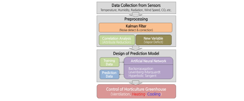
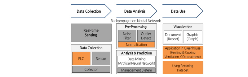
Therefore, this study proposed a greenhouse internal temperature prediction model using an ANN to precisely control the greenhouse environment (Fig. 1). The data preprocessing used the Kalman filter to reduce the noise and measurement error and correlation analysis to improve the accuracy of the prediction model by data reduction and extraction of new factors to be reflected in the training data. In addition, a Multiple Regression Model (MRM) and Recurrent Neural Network (RNN) were constructed and compared to the performance of the ANN. The prediction model proposed for greenhouse ventilation control was applied for effective greenhouse energy management, thereby reducing the energy cost of the greenhouse.

Fig. 1. Frame of management system for greenhouse: Data collection, preprocessing, design of prediction model using ANN, and control of greenhouse.

Materials and Methods

This study was conducted on a greenhouse in the Protected Horticulture Research Institute in Haman, Gyeongsangnam-do in Korea. Various types of data were collected from environmental sensors, which were located in the greenhouse and used for controlling the greenhouse. A large amount of data was selected and analyzed to control the greenhouse effectively, reducing energy consumption and increasing production.

Greenhouse Conditions

The data were collected from a Venlo-type greenhouse. The heating conditions were set to 20°C during the day (09:00-18:00) and 18°C at night (18:00-09:00). The ventilation conditions were set for a target temperature of 25°C during the day, with a tolerance of 2°C, and 19 °C at night, with a tolerance of 3°C. The tested crops, paprika ‘Cupra’ and tomato ‘Deafness’, were transplanted on July 26, 2016. For ventilation, a ventilation window was opened when the temperature reached 28°C or higher. The main heater of the greenhouse was a diesel boiler supplying hot water, and a gas engine heat pump (GHP) was used as the auxiliary heater and cooler. For data collection, a temperature and humidity sensor (111N & 222N, Jauntering Int., Taiwan), carbonic acid sensor (VT-250, SOHA Tech, Korea), solar radiation sensor (CNR4, KIPP&ZONEN, the Netherlands), and data logger (CR1000, Campbell Scientific, USA) were used under a radiation shield condition.

Data Collection and Preprocessing

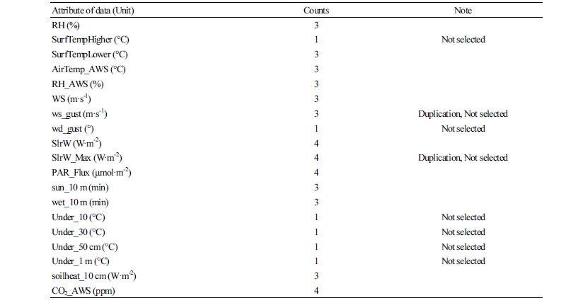
The collected environmental measurement data included 28 items including greenhouse temperature, relative humidity, solar radiation, wind speed, rainfall, surface temperature, external CO₂ concentration and so on (Table 1). The data collected for one year in 2016 were used for analysis, and 10-minute average values were used because the variation in the data was small. The data preprocessing is as follows.

1. Select the data for greenhouse control

2. Correction of data noise and outlier using Kalman filter

3. Correlation analysis between internal temperature and other factors

4. Calculate and extract the vapor deficit as a new factor

Table 1. Collected data of greenhouse: Data were collected from various sensors such as external weather condition, radiation, humidity, wind speed, etc.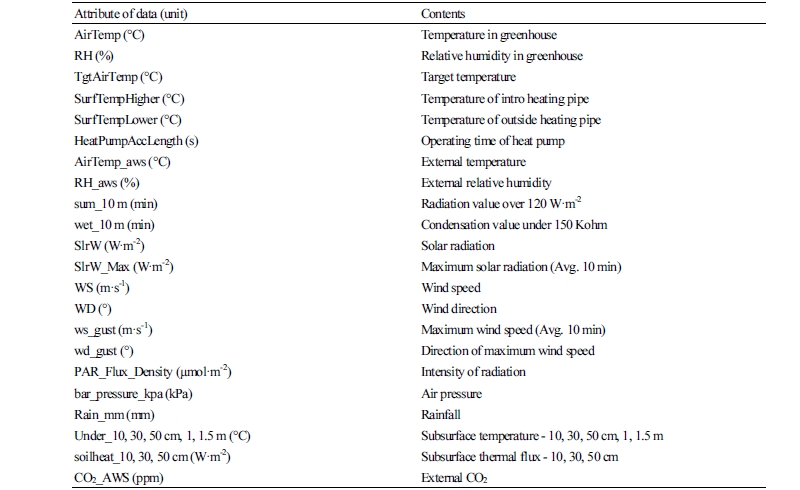

Kalman Filter

The Kalman filter was used to compensate for the data noise due to automatic control malfunction, manual operation, and sensor measurement error. The Kalman filter (Gerrit et al., 1998; Kalman, 1960) analyzed the measured values that contain the noise with the least squares method and predicted the value after the specific time for revision (Fig. 2).

Fig. 2. Concept of Kalman filter: The filter is divided into two parts as time update and measurement update.

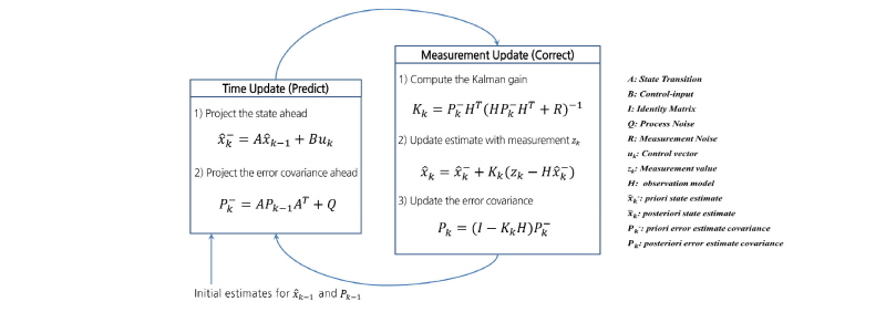
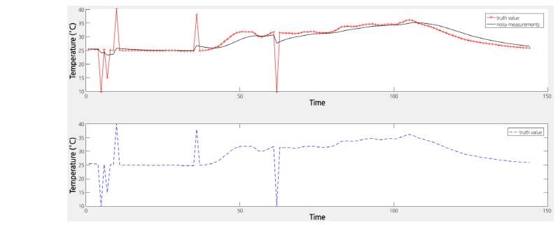
The Q (process noise) value represents an error which is related to an external factor, and the R (measurement noise) value represents a measurement error. The external factor is the outlier of the measured value due to the malfunction of the automatic control and the manual control. The measurement error is shown in Table 2, which includes the error ranges of the sensors and the data logger. Noise was removed by applying a Kalman filter to each measured value (Fig. 3).

Table 2. Error range of measured values

Fig. 3. Noise calibration by Kalman filter.

Data Reduction by Correlation Analysis

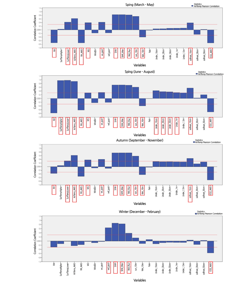
The variable subset selection techniques include the filter method, wrapper method, and embedded method. The filter method was selected using correlation analysis to solve the problem of multicollinearity that can occur when using the final model in the real environment. The correlation of the greenhouse temperature with collected data was analyzed to improve the accuracy of the prediction model and reduce the input variables (dimension reduction). The Pearson Correlation Coefficient method was used for the correlation analysis, and only one variable that had the same or overlapping correlation coefficient was selected. Out of 28 variables, 11 variables, which had a correlation coefficient of 0.3 or higher or -0.3 or lower, were selected (Table 3 and Fig. 4).

Fig. 4. Seasonal correlation analysis of internal temperature and other factors

Table 3. Selection factors by correlation analysis, 11 factors

Construction of Training Data Set and Prediction Models

The training data set was constructed based on the measured data for learning by the prediction model. The relative humidity was not used for statistical analysis or greenhouse control. Instead, the vapor pressure and vapor deficit were used for greenhouse control. Therefore, the vapor deficits inside and outside the greenhouse were calculated and used as the input variables for the ANN model. The following equations were used to calculate the vapor deficit.

The data were divided into seasons in spring (March - May), summer (June - August), autumn (September - November), and winter (December - February). Each seasonal dataset was composed of 10-min averages, totaling 52,575 samples with 13,249 samples, 13,248 samples, 13,103 samples and 12,975 samples, respectively.

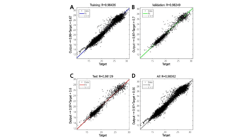
The training data set for the ANN model was constructed through a series of processes and classified by season. It consisted of 11 variables, and 70% of the training data sets were used for learning while the other 30% were used for model verification (Table 4). The internal temperature was the target variable, and the measured value and the predicted value were compared using 2017 data by season.

A MRM was constructed to compare the performance of the developed ANN model using the same training data set. The internal temperature of the greenhouse was the target variable, while all other variables were the independent variables. The R-squared values of spring, summer, autumn, and winter were 92.7, 98.6, 90.3 and 86.3, respectively. Table 5 shows the summary of models.

Table 4. Training data set for prediction model: Data are selected as total 11 variables including the vapor deficit without duplication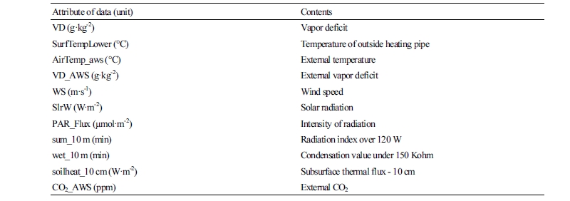

Table 5. Summary of regression models constructed by season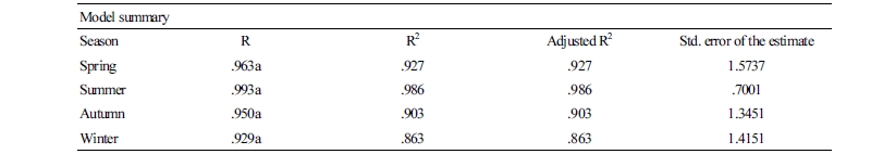

Predictors: (Constant), CO2_AWS, SurfTempLower, Wet_10 m, WS, VD, sun_10 m, soilheat_10 cm, VD_AWS, PAR_Flux, AirTemp_AWS, VD, SlrW

Table 6 shows the correlations that indicated the impact of other variables on the greenhouse temperature, which was the dependent variable. The vapor deficit, temperature of outside heating pipe, external temperature, external vapor deficit, wind speed, solar radiation, intensity of radiation, radiation index over 120 W, condensation value under 150 Kohm, subsurface thermal flux-10cm, and external CO₂ showed a correlation with internal temperature of the greenhouse. The MRM equation is shown below (Table 7).

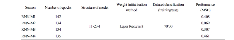
The RNN has difficulty learning due to the vanishing gradient problem of time series data. Another disadvantage is that learning time is longer than for the backpropagation algorithm. In order to compare the performance of the RNN with the proposed model, the RNN model was constructed with the same training data set (Table 8).

Table 6. Coefficients of regression models

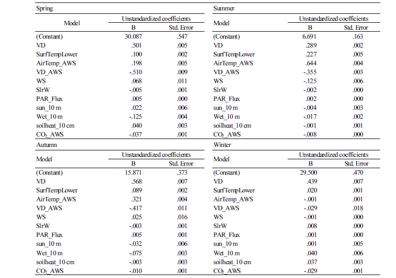
Table 7. Coefficients of multiple regression models used for the equation (2) as marked from C1 to C12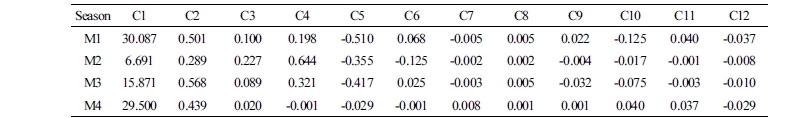

M1: Spring, M2: Summer, M3: Autumn, M4: Winter.

Table 8. Recurrent neural network (RNN) model

M1: Spring, M2: Summer, M3: Autumn, M4: Winter.

Construction of Artificial Neural Network

In order to construct and analyze the prediction model, the study was conducted in the following development environment. The processor was an Intel (R) Core (TM) i3-5005U @ 2.0GHz, RAM was 8GB, and the system was based on Windows 10 64 bit. MATLAB (R2016a) was used for constructing models. NN toolbox was used and re-coding for selecting neural network type (backpropagation or layer recurrent).

The backpropagation algorithm, which was one of the supervised learning techniques, was used for modeling with the hidden layer to improve the prediction rate of the model (Fig. 5). The ANN featured outstanding performance since each neuron calculates the weight factor in two stages. The Levenberg-Marqardt algorithm (Christian et al., 2004; Lourakis, 2005) was used for the learning technique. The algorithm combined the Gauss-Newton technique and Gradient Descent technique. The algorithm obtained the value with the Gradient Descent technique when the prediction was far from the value and with the Gauss-Newton technique if the prediction was near the value. The hyperbolic tangent was used as the activation function for the continuous differentiation of weight factors of the ANN. The hyperbolic tangent seems to be more suitable than other activation functions for greenhouse data since the range was -1 to 1.

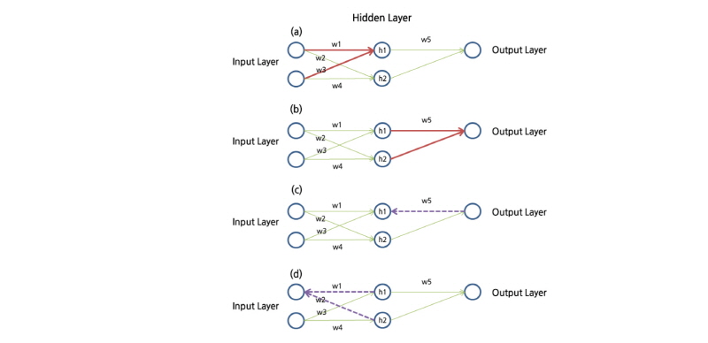
Fig. 5. Concept of backpropagation algorithm: a) Calculation of h1 layer’s weight by w1, w3, b) Calculation of output layer’s weight(w5) by h1, h2 of weights, c) Update weight of w5 based on output, d) Update weight of w1, w2 based on h1, h2 layer’s weight, e) Repeat once more in the forward direction.

Table 9. Comparison of RMSE for ANN structures

Previous studies have not used an ANN technique for ventilation control. Although we used a general method for model learning (Levenberg-Marqardt), it was considered to be sufficient for constructing the model because it has better performance than other learning methods.

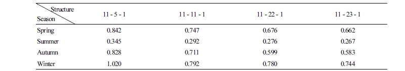
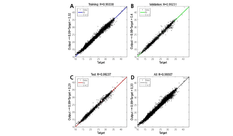
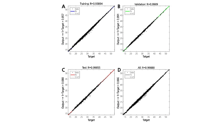
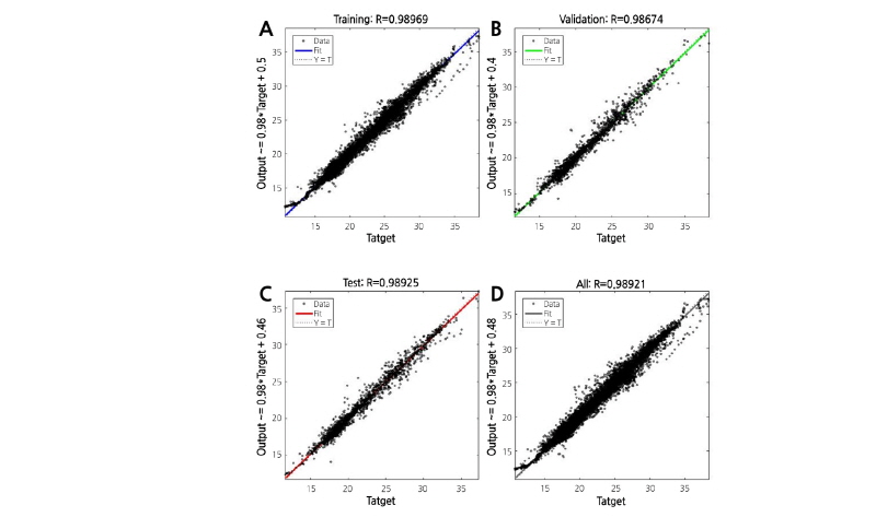
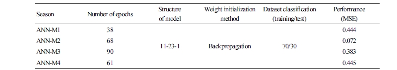
The hidden layer number of the ANN was set to n/2, n, 2n, and 2n+1 when the number of input data was n (Zhang, 1998). The structure of the ANN was selected based on the smallest values of Root Mean Square Error (RMSE) criteria (Table 9). The hidden layer number with the smallest RMSE value was 23. Seasonal models were also constructed (Figs. 6, 7, 8, 9). Table 10 shows the architecture and learning conditions of the model.

Fig. 6. Training results of spring: (A) Training, (B) Validation, (C) Test, and (D) Comprehensive results.

Fig. 7. Training results of summer: (A) Training, (B) Validation, (C) Test, and (D) Comprehensive results.

Fig. 8. Training results of autumn: (A) Training, (B) Validation, (C) Test, and (D) Comprehensive results.

Fig. 9. Training results of winter: (A) Training, (B) Validation, (C) Test, and (D) Comprehensive results.

However, considering the hardware performance of the greenhouse control system (PLC: programmable logic controller) and the speed of the algorithm, the well-known algorithm (backpropagation) was used to construct the ANN. Backpropagation is more appropriate to apply to the greenhouse control system than the latest algorithms that exhibit slow learning and processing speeds.

Table 10. Comparison of seasonal ANN models

M1: Spring, M2: Summer, M3: Autumn, M4: Winter.

Results and Discussion

The prediction model based on the ANN can perform climate control by predicting the internal temperature of the greenhouse for ventilation so that the control range of the P-band can be determined.

Comparison of the ANN Model with the MRM and RNN

The performance of the seasonally constructed ANN, MRM and RNN models using the backpropagation algorithm was analyzed and compared. We used the RMSE values to compare the measured values and predicted values seasonally and analyzed the prediction performance.

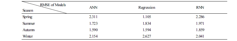
Compared to the ANN, the MRM had difficulty rapidly predicting the changing internal temperature. And the prediction accuracy of the MRM was worse than the ANN, although the patterns of the predicted value and measured value were similar. In addition, the RNN showed similar prediction performance as the proposed model (Fig. 10). Since the ANN had a smaller RMSE value than the other prediction models, it can be concluded that the ANN greenhouse temperature prediction was more accurate (Table 11).

Fig. 10. Comparison of prediction models: (A) spring, (B) summer, (C) autumn, and (D) winter.

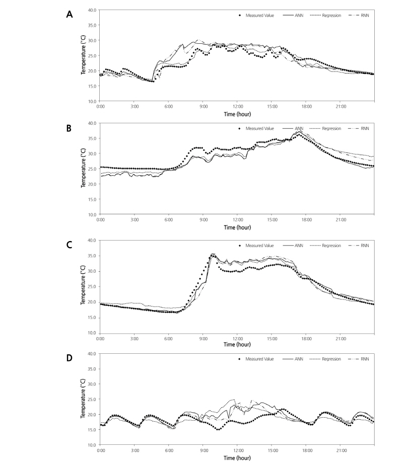
The RNN model took double the learning time as the proposed model and was slow and heavy in applying software to the control system (PLC) in the greenhouse. There was also no apparent difference in prediction performance compared with the ANN model. Therefore, it can be concluded that the proposed model is more effectively applied to a greenhouse control system that uses low-performance hardware.

Table 11. Comparison of seasonal RMSE of prediction models

Application of Proposed Prediction Method

The ventilation window of the wind side and downwind side was separately operated for ventilation control, and the opening of the ventilation window could be manipulated by 0-100%. The P-band was used to calculate the open position of the ventilation window.

This represents the range of temperatures that corresponds to the excess of the set temperature for opening the window 100%. The controller increases the window opening by 20% each time the temperature increases 1°C from the set temperature. The controller operates more sensitively as the size of each step increases when the P-band decreases. Moreover, the P-band is set differently according to the season. The P-band is set large in the winter so that the ventilation window operates slowly while it is set small in the summer so that the ventilation window operates quickly to control the greenhouse temperature. Therefore, the greenhouse temperature data predicted by the ANN model applied to ventilation control opens or closes the ventilation window in advance to minimize the loss of greenhouse energy.

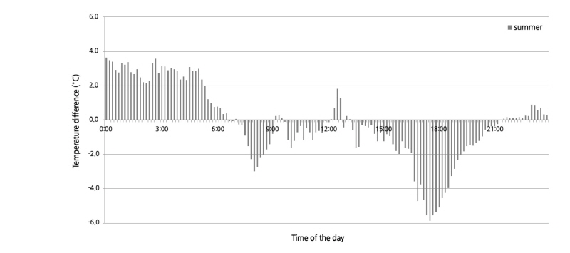
The proposed prediction model can estimate the temperature difference inside and outside of the greenhouse from the predicted internal temperature and the determined control range of the P-band. The P-band was set differently for each season. When the temperature difference is large, it is possible to rapidly ventilate using the big band range. On the other hand, the energy loss of the greenhouse can be minimized by reducing the band range (Fig. 11).

Fig. 11. Temperature difference inside and outside of the greenhouse in summer: In this case, there is a negative temperature difference during daytime, and the P-band should be controlled for ventilation.

Discussion

This study predicted the internal temperature using the backpropagation algorithm based on the data collected from a Venlo-type greenhouse. This predicted temperature can be then be applied to the greenhouse ventilation to control the greenhouse more efficiently. The proposed model was verified by comparing the performance of the MRM and RNN models.

Fig. 12. Application of data mining techniques in horticulture: Data mining techniques can be applied to agricultural fields in a variety of ways such as pattern analysis and classification techniques.

Although earlier studies used data measured by the sensors, they did not consider the measurement error or manual and automatic operating error. Also, it was not suitable to apply the proposed model or method from these previous studies directly to greenhouse control or cultivation. So far, no study has been conducted to control the ventilation of greenhouse using an ANN.

In this study, the Kalman filter was used to remove the measurement error and noise to ensure data reliability. Prediction performance was improved by using correlation analysis to extract variables that correlated with the temperature in the greenhouse. As a result, the RMSE of the ANN, MRM and RNN models were 1.723, 1.834 and 1.971 respectively in the summer. The ANN model was judged to be more accurate than other prediction models since its RMSE value was smaller. The RNN model showed similar patterns and prediction performance to the ANN model, but it required double the learning time, and it is not suitable considering hardware and software specifications used for general greenhouse controllers. In addition, the predicted temperature can be applied to the ventilation control, thereby allowing the P-band to change more quickly. If the temperature difference between the inside and outside of the greenhouse is large, the P-band was enlarged, allowing the ventilation to be faster. It is possible to reduce the energy cost and minimize energy loss in the greenhouse by using a smaller P-band range.

However, the experiment was only carried out in a Venlo-type greenhouse, making the results difficult to apply to other types of greenhouses, such as plastic greenhouses. Therefore, it is necessary to consider these physical conditions when constructing the prediction model. Further studies can utilize this method to predict the greenhouse heating load to reduce the energy consumed by the greenhouse and manage the energy more efficiently to reduce costs. Moreover, the study enables the data mining technique to be applied to agriculture in various ways (Fig. 12).