Introduction

The proportion of farms utilizing greenhouses has grown, and studies are actively being conducted both domestically and abroad in order to improve greenhouse crop yield and increase farmers’ profits. A greenhouse can provide the optimal environment for crops regardless of the season because the conditions of the indoor environment are less affected by outside weather conditions and can be controlled. Among the indoor environmental conditions, temperature is the most important to manage because it directly affects the growth of crops (Lee et al., 2019; Qian et al., 2015). When the temperature inside the greenhouse surpasses the proper temperature range for crop growth, cooling of the greenhouse is required. Opening the ventilation windows to let outside air in is the primary method used to lower the temperature inside the greenhouse.

Unlike other controlled factors, controlling ventilation requires precision management because it is directly affected by outside environmental conditions. Ventilation is typically accomplished by controlling the opening of windows to let in the colder outdoor air to reduce the greenhouse temperature (Kim et al., 2014; Pahuja et al., 2015; Castañeda-Miranda and Castaño, 2017). The ventilation speed is affected by the amount the window is opened, the difference between the indoor temperature and the outside temperature, and the outdoor wind velocity and direction (Simons and Waters, 2002). Among these effects, the outdoor temperature and wind conditions cannot be manipulated and can only be monitored. These factors act as disturbances that strongly affect the control logic, so they make it difficult to control ventilation.

In order to control ventilation more precisely, many studies have been performed to design control systems by designing a model through the interpretation of physical phenomena occurring in the greenhouse (Villarreal-Guerrero et al., 2012; Hong and Lee, 2014; Montoya et al., 2016; Li et al., 2018). Such models can be classified into two types. The first type is the greenhouse model, which is also known as the ventilation model. This model predicts the ventilation performance and changes in the greenhouse environment based on weather factors or other necessary environmental factors (Youssef et al., 2011; Benni et al., 2016; Montoya et al., 2016). This method uses control logic based on either the modeling created by formulating the flow of material properties according to the law of conservation of physical energy or the experience- based empirical modeling of the greenhouse. Furthermore, the response between the actuators and variables is due to the greenhouse characteristics, and the influence factor based on other environmental factors is very large. Hence, most studies conducted simulations (Zeng et al., 2012; Rodríguez et al., 2015). The other model is the evaluation model. In this model, various operation scenarios for the ventilation system are simulated using a virtual greenhouse, and the best solution is selected from the simulation results. The computational fluid dynamics (CFD) is an example of such a model (Benni et al., 2016; Norton et al., 2007). By using this modeling technique, it is possible to verify the ventilation strategy as well as the feasibility of precision control of the greenhouse environment in general; however, this model has not been considered for commercial products due to practical limitations (Park et al., 2015). For example, commercial control boards have limitations in computing non-linear models, which require complex computations or cannot be interpreted using polynomial analysis. Modeling analysis methods involving structural analysis in the CFD field is another example. Also, when factors that are difficult to measure using sensors, such as the biological characteristics of leaf area index and amount of evapotranspiration, are used as the model’s variables, the commercial control boards are not capable of handling such models.

Under these circumstances, the control logic employed by the integrated climate control systems for the greenhouse, which is currently commercially available, is simple. However, the control logic has been developed to accommodate various environmental variables. The advanced greenhouse operating systems have proposed index criteria for heating load and ventilation load, and these systems employ a variety of elaborate experience-based models. These models make appropriate decisions based on the crop growth data and greenhouse environmental information, which have been accumulated over the past several decades (Yang et al., 1989). However, in countries with different climate conditions, the optimal value of coefficients used in proportional band (P-band) control must be obtained using a trial and error method, or farmers can operate the greenhouse control system using their own established knowledge. Domestically, commercial products that utilize logic based on the P-band are being developed. The P-band control uses a simple linear model that applies to the influence coefficients, which reflects the other environmental factors to the target environmental factor. Solar radiation, outdoor temperature, and wind speed are commonly used as the influence factors for ventilation control. However, it is very difficult to determine intuitively what the exact values should be for these influence coefficients and whether they are negative influences or positive influences.

To find these conditions, experimental statistical methods are widely being used (Majdi et al., 2019). Among these methods, the surface response methodology (SRM) identifies the optimal coefficient through various experimental conditions (Thakur et al., 2018). This method can minimize the number of scenarios for the experiment, so it is widely used in many fields (Kaushal et al., 2015). In addition, the SRM is frequently used for tuning in coefficients of a proportional integral derivation (PID) controller for many applications (Nakano and Jutan, 1994; Demirtas and Karaoglan, 2012). Research on the optimization of coefficients for greenhouse environmental control using an experimental statistical approach is required, but it is very rare to find actual results from such studies. For greenhouses that utilize natural sunlight, the optimized influence coefficients by time must be determined. The daily changes in the greenhouse environment have a certain pattern. When each day was carefully observed, the indoor temperature began to rise from sunrise, and the heat inside the greenhouse tends to accumulate excessively in the afternoon. Also, the temperature inside the greenhouse before sunset drops drastically, so the heat cannot be preserved overnight (Blasco et al., 2007; Kwon et al., 2013). Therefore, a day can be divided into sunrise, sunset, noon, and midnight, and different strategies must be planned for different time slots to control the greenhouse environment. A commercial integrated climate control software system for greenhouses should allow the user to change the settings for each time slot, and there is a need for finding the optimal influence coefficients for each time slot.

In this study, the proportional derivative band (PD band) control technique was introduced as the logic for controlling the greenhouse ventilation. In order to optimize settings for this control logic, research was conducted to obtain the influence values for the solar radiation, outside temperature, and wind speed, as well as the values for the optimal influence coefficients for the P-band and D parameters. Thirty-two experimental conditions were derived from the response surface analysis, and a day was divided into six time slots so the coefficients could be optimized for each time slot. Ultimately, this paper proposes a very simple and efficient method for temperature control through ventilation in the greenhouse and discusses the tendency of optimal coefficients through each time period.

Materials and Methods

Description of the Experimental Greenhouse

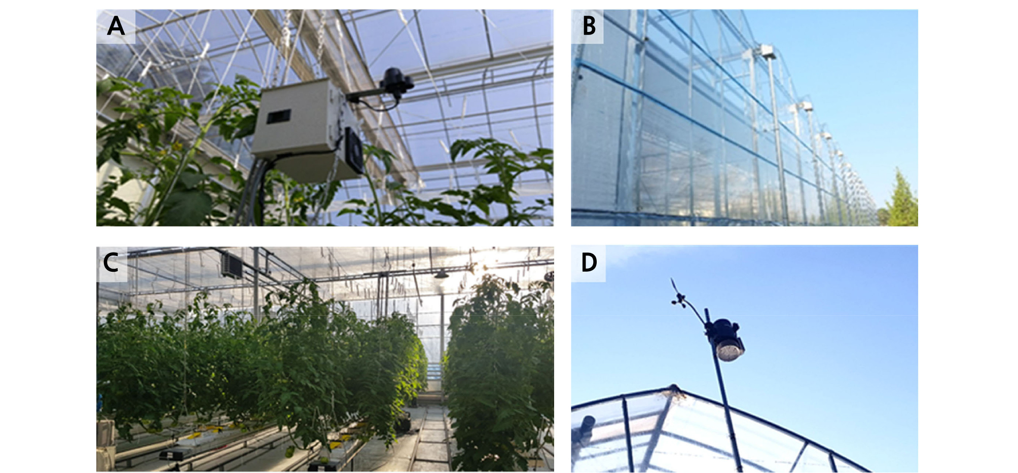
An experimental greenhouse at Korea Institute of Science and Technology, Gangneung, which is a multi-span Venlo-type structure, was used for the experiment. The size of each unit is 16 m in length and 12.5 m in width, and a total of four units has been connected (Fig. 1A and 1B). The crop used in the experiment was ‘Dafnis’ tomatoes (Solanum lycopersicum L.). The experiment was conducted 6 months after the tomato seedlings were transplanted and when the 15th flower cluster had bloomed (Fig. 1C). The inside sensor module was located at the center of the greenhouse (Fig. 1A), and every minute, the average value of the data collected every ten seconds was saved to the database. The sensor module (JN-DL1, Jinong Inc., Gyeonggi-province, Republic of Korea,) measured the temperature, humidity, and CO₂ concentration inside the greenhouse. Outside conditions were measured by a weather station (Vantage Pro 2 DS6450, Davis Instrument, California, United States) which provides information of outside temperature, solar radiation, and wind velocity (Fig. 1D). The experimental greenhouse was operated using an algorithm developed in-house.

Fig. 1.

The sensors for monitoring the environment inside the greenhouse (A), outside view of the vinyl-type multi-span Venlo-type greenhouse (B), tomato plants growing inside the greenhouse (C), and weather station to measure outside climate values (D).

Hardware and Software System

The control system used in this experiment was divided into open source hardware and software. The hardware was manufactured in modules, and necessary modules can be added on top of the basic module, known as a baseboard, in a stacked manner. The controller consists of the baseboard and three other modules, which can function as the sensor node or actuator node depending on the combination of the modules. The software program that operates the individual nodes was installed on a Raspberry Pi, and the overall system operated through the communications between the Raspberry Pi and the baseboard. Fig. 2 shows the controller configuration.

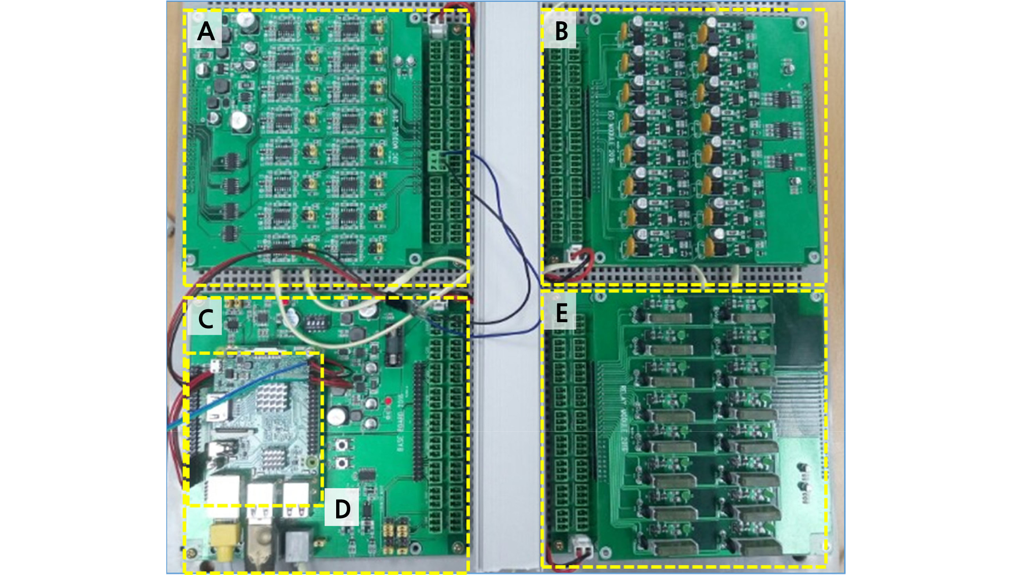
Fig. 2.

Environmental controller configuration. ADC module (A): connected to the baseboard and is used to measure the voltage, current, and resistance. ISO module (B): connected to the baseboard and detects a contact input. Baseboard (C): basic CPU board that uses ARM32F407, and independent modules can be installed on it. The baseboard establishes communications between the modules and connects the input signal. Digital board (D): combination of the baseboard and the Raspberry Pi 3 board, which runs on Linux OS and processes sensors for communications (232,485) and counter (wind direction, wind speed) sensors. Relay module (E): connected to the baseboard and generates a contact output.

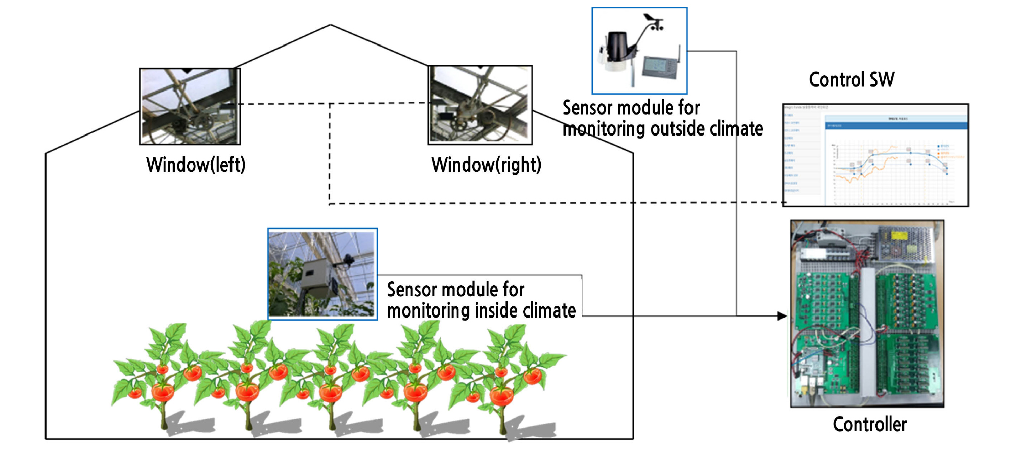
The overall system operated as shown in Fig. 3. The outdoor and indoor environmental data were collected through the weather station and the sensor node inside the greenhouse, respectively. The collected data were sent to the main controller every minute using a standard transmission protocol. The transmitted data were stored on the database, and the control algorithm program generates operation commands for the actuators based on these data. The generated commands are then sent to the controller, and the controller sends the signal to the relays to operate the actuators. The control program is an integrated greenhouse climate control algorithm that was developed in-house for this study. Rule-based operations can be performed for both P-band- and PD-band-based algorithms using this program.

Fig. 3.

Overview diagram of the PD-band control system, which monitors and controls the greenhouse climate.

PD-band-based Control Logic for The Ventilation Control

The proportional control band is a control logic widely used in integrated greenhouse climate control systems. In this logic, the controller can decide how much the ventilation window is opened on a scale from 0% to 100%. For example, when the greenhouse temperature is measured, the ventilation window is opened to a degree proportional to how much the actual temperature has exceeded the set temperature. Here, P-band is required to calculate the opening position of the ventilation window. The P-band indicates the excess temperature over the set temperature that would require the window to be opened 100%, and this value is expressed in Celsius. Therefore, once the greenhouse temperature exceeds the set temperature, the window is opened by a certain percentage each time the greenhouse temperature rises by 1°C.

Formula [1] shows the formula for calculating the band value. Also, the speed at which the heat and humidity are removed through ventilation is determined primarily by the outside temperature and the wind velocity. The outside temperature is low, and the wind speed is strong in the winter, so the heat or humidity is quickly removed. However, during the spring or early summer when the outdoor temperature is high and the wind speed is relatively weak, it takes a long time to remove the heat or humidity. In order to control ventilation seamlessly, the excess heat or humidity must be removed at a proper speed (Fitz-Rodríguez et al., 2010). If the greenhouse ventilation is performed too cautiously, it will take longer to remove the heat or humidity, and the heat or humidity will rise as a result. In this case, a relatively small P-band is advantageous. However, if the P-band is set too small during the night when the heat needs to be preserved, the heat or humidity may be removed too quickly so the ventilation performance will degrade. To remedy this issue in advance, the time differential values of the set value and the target value were added as constants to respond to the changes in the error.

where X₁ ‑ X₅ are influence coefficients, PB is the bandwidth index, R_m is the maximum solar radiation (set value), R_c is the current solar radiation (measured value), T_om is the maximum outside temperature (set value), T_oc is the current outside temperature (measured value), V_m is the maximum wind speed (set value), V_c is the current wind speed (measured value), T_c is the current indoor temperature, and T_t is the current target temperature.

Design and Experiment for The Response Surface Analysis Method to Optimize Ventilation Conditions

The response surface analysis is suitable for fitting a quadratic surface, and it helps to optimize the process parameters with a minimum number of experiments as well as to analyze the interaction between the parameters (Betiku and Taiwo, 2015). In addition, the characteristics of the response surface analysis are that information can be distributed across the entire experimental region, residual and prediction errors are minimized, and a high level of examining compatibility lack is exhibited. Models can be designed sequentially from a simple model to a high-order model. The combination of factor levels used is minimized, so graph analysis can be performed using simple data patterns. Minitab 17 (Eretec Inc., Korea) was the program used in this study. Minitab 17 is equipped with the necessary tools to prepare data for analysis and derive results through analysis. The response surface methodology analysis was conducted to optimize the five influence factors X₁ ‑ X₅ for the PD-band control. In this analysis, the central composite design (CCD) was created in a grid pattern. The CCD is able to adapt to the full quadratic model of the response surface design. The experimental group created through the design of the CCD model are summarized in Table 1.

Table 1. Experimental design using a central composite design (CCD) model of 32 trials

In this ventilation control experiment, the result for one sample was used as the response value by taking the RMSE difference of the temperatures collected during one day of greenhouse operation. The entire experiment lasted from April until May 2017. The spring weather condition was chosen because the reduction in temperature through ventilation is much needed during this period. Excluding the rainy days, the experiment was conducted over a total of 32 days. In addition, a day was divided into six time slots, and the greenhouse control time slots were defined as P₁ through P₆. These time slots were reflected in the results, and the optimization coefficients for each time slot were compared (Table 2).

Table 2. Time slots for the greenhouse climate control operation and the target temperature through ventilation for each time slot

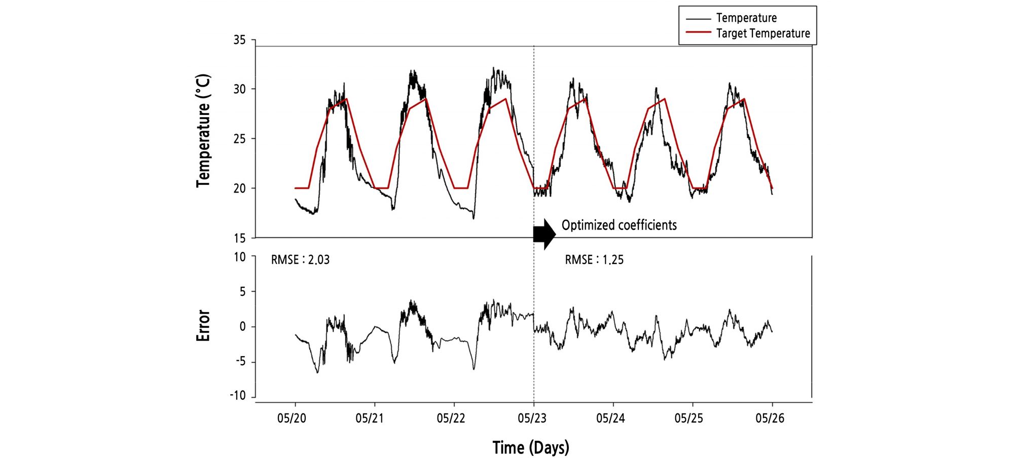
To validate the optimal coefficients, validation experiments were conducted to compare the control performance with the optimal setting and the default setting. When the default setting was used, values 5.0, 1.0, ‑1.0, 1.0, and 0 were used from X₁ to X₅, respectively. Ventilation control based on these values was performed from May 20 to May 22. After that, the ventilation experiment was carried out by applying the optimization coefficients obtained by response surface analysis (from May 23 to May 25).

Results and Discussion

Design and Experiment for the Response Surface Analysis Method to Optimize Ventilation Conditions

The PD-band ventilation control experiment was conducted over 32 days between April 2017 until May 2017-on days when it was not raining. The coefficient value was designed using the response surface analysis method, and it was provided as an input each day. The 32-sample data shown earlier in Table 2 were divided into 6 equal parts, and the RMSE value between the target ventilation temperature and the actual temperature for each time slot was used as the response value. The target ventilation values were divided into linear intervals for each time slot and compared with the measured values using 1:1 comparison to compute the RMSE values. These results can be seen in Table 3. Also, according to the plan for the response surface analysis experiment, which was designed for the purpose of finding the optimal parameters for the ventilation settings, characteristics of the following parameters were investigated under each specified condition.

Table 3. Experimental design using the CCD model of 32 trials with the RMSE as response

Results of the Linear Regression Model

The regression equation of second order [3] for the RMSE for the target ventilation value was derived by assigning the experimental results as the objective function of the response surface regression equation. This equation was calculated by separating the coefficients P₁ ‑ P₆ for each time slot and the results, and the calculation results are shown in Table 4. Values for 20 coefficients were obtained using analysis of variance (ANOVA), and 95% reliability was required for the analysis (p < 0.05).

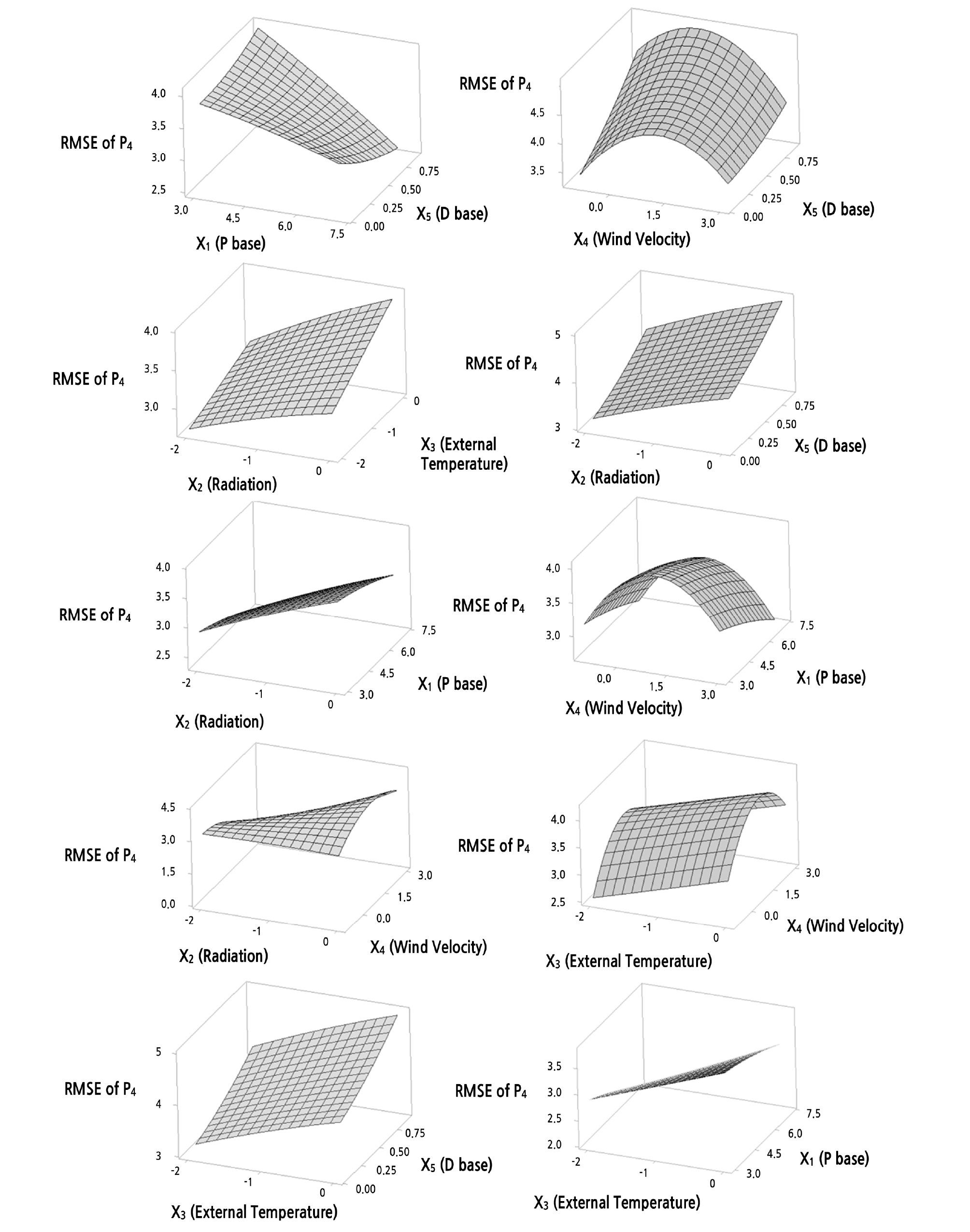
The data in Table 4 were analyzed using the response surface optimization method, and the results were displayed using 3-dimensional surface contour plots, similar to the ones shown in Fig. 4. Fig. 4 shows the contour plots for the P₄ time slot, which is when solar radiation is at the highest and the reduction in temperature is most needed due to the heat accumulated in the afternoon. This time slot is the most important period for ventilation control (Villarreal-Guerrero et al., 2012). Here, the correlation between two influence factors can be verified. X₂ and X₃ are coefficients for the outdoor solar radiation and outside temperature, respectively, and it is shown that the more negative the influences of the two factors are, the lower the RMSE distribution is. This result can be attributed to the fact that the bandwidth is reduced in this period to increase how much the ventilation windows are opened because the temperature is more often higher than the target ventilation temperature during the P₄ time slot. This pattern is also shown in the graph of the correlation between solar radiation (X₂) and the coefficient of the differential error (X₅), as well as in the graph of the correlation between the outside temperature (X₃) and the bandwidth constant (X₁). For the coefficient of wind speed (X₄), correlation with all other influence coefficients yielded a second order polynomial relationship.

Table 4. Coefficients P₁-P₆ of the regression model of second order obtained through the response surface analysis method

Fig. 4.

Response surface plots with two factors to RMSE of P₄.

Results of the Surface Response Analysis for Optimizing the Coefficients

The optimal values for the control influence coefficients (X₁ ‑ X₅) were obtained for each time slot (P₁ ‑ P₆) using the results of the surface response analysis method (Table 5). When the influence values for each time slot were examined, the influence values for the outdoor solar radiation and outside temperature were either zero or very small for the P₁ and P₆ time slots. These time slots correspond to night time, so there is no outdoor solar radiation, and the outside temperature does not vary much. Also, the analysis results showed that the influence due to solar radiation (X₂) is negative. This result is attributed to the fact that the bandwidth is reduced to lower the temperature quickly because the greater the solar radiation value is, the greater the effect of solar radiation on the rise of the indoor temperature. A similar phenomenon can be observed for the influence of the outside temperature (X₃). The influence of the wind speed (X₄) is primarily positive, but it does not appear to be a first order linear relationship, as was verified by the 3-dimensional surface contour plots. The index for the influence (X₅) of the changes in the error exhibits a positive influence. Other than the P₁ time slot, this value was 0.9 for all other time slots. This result indicates that three values (0.3, 0.5, and 0.7) for the influence coefficient, which were used in the previous experimental design, were rather low. This result also shows that responding to changes in the temperature deviation is an important element. In the existing climate controller, factor X₁ was non-existent. Therefore, it seems that low values were used during the experimental design because default values for this factor were not available. In the case of X₂ and X₃, the optimum convergence was at ‑ 2.0 in the P₃ ‑ P₅ time slot. However, since this is the minimum range in the experimental design, there is a possibility that an optimal value can be derived from a lower value, and it will be possible to apply a lower value than ‑2.0.

Table 5. Optimal influence coefficients per time slot obtained through the surface response analysis method for optimizing ventilation control

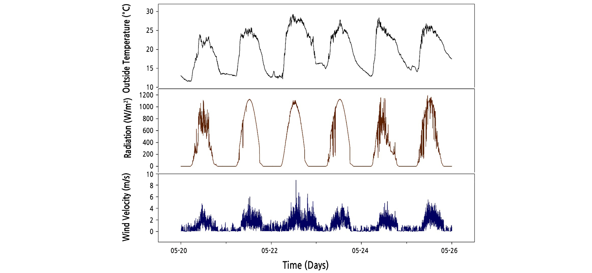
The derived optimal coefficients were entered into the real system, and the operation of the greenhouse ventilation control was verified. The optimal coefficients were set for each time slot, and the ventilation control was performed to control the greenhouse temperature for three days. Fig. 5 shows the temperature changes of the greenhouse before and after the application of the optimal coefficients. Fig. 5 (top) shows the temperature change and the set temperature value, and the bottom of the graph shows the difference between the two values. For comparison, the temperature control performance through the optimal ventilation coefficients produced an RMSE value of 1.25°C for the target temperature. When the experimental design method was conducted for approximately one month, the RMSE value of 2.03°C was obtained for the average temperature. Therefore, in comparison, the 1.25°C RMSE result verifies improved performance. In particular, the ventilation control performance was excellent in the time slots P₃ and P₅, when the temperature changed more drastically. As for the P₄ time slot, it seems there is a limitation in controlling the temperature through ventilation. For a period, such as this, a fogging method can be used to cool down the greenhouse. Fig. 6 shows the change in outside environmental conditions in this experiment. The changes in outside temperature were similar, and the maximum solar radiation values had similar patterns during this experiment. On May 25th, the inside temperature of the greenhouse was lower than on a typical day because of cloudy and rainy weather from noon to afternoon. Through this data, a sudden temperature change occurs in the greenhouse at sunrise and sunset, but a relatively gradual change of temperature was observed in the optimum coefficient experiment. Therefore, the performance of the ventilation PD band control logic corresponding to the outside environmental conditions has been confirmed in this study.

Fig. 5.

Temperature changes in the greenhouse managed using the optimal ventilation coefficients and comparison with the target ventilation temperatures.

Fig. 6.

Changes in outside environmental conditions in the experiment with optimal ventilation coefficients.

Conclusions

In this study, a PD-band control method was proposed for controlling greenhouse ventilation to manage temperature, and its performance was verified. To optimize the settings (influence factors) for the PD-band, a response surface analysis method was conducted, and the experimental statistical method was performed. Based on the results, conditions for the optimum ventilation control were investigated. In order to optimize the influence factors such as solar radiation, the outside temperature, wind speed, P-band width, and D coefficient, which were required for PD-band ventilation control, 32 experimental conditions were designed using the experimental design method. The values for each factor were applied to real greenhouse ventilation operation, and the response values were obtained using the RMSE difference of the target ventilation temperature. The greenhouse operation hours were divided into six time slots, and the response values were used to obtain the optimized coefficients for each time slot. By using ANOVA analysis, a second order polynomial formula was derived, and results were obtained for each time slot. Lastly, in order to minimize the RMSE, the optimum coefficients for the influence factors were calculated, and these values were applied to a real greenhouse system. The ventilation control performance was evaluated, and the RMSE value of 1.25°C confirmed a performance improvement due to the optimized coefficients. It showed that optimized parameters were successfully applied to ventilation control and obtained better performance. However, experiments must be conducted over a long period to obtain the coefficients, and there is a concern that the optimization is specific to the greenhouse used in this experiment. Hence, it is necessary to consider a method to reduce the duration of the optimization experiment.

This study proved that environmental settings, which are typically determined by the greenhouse operator’s skills and experience, can be optimized through a statistical approach. It is anticipated that the study results will be useful in providing the numerical guidelines for the influence factors of ventilation control settings. In addition, it can be very useful for automatic control of appropriate setting values according to various external weather changes or several ventilation periods in a day.