

Introduction
Materials and Methods
Study Site Description
Experimental Design and Land Preparation
Crop Seeding and Transplanting
Management Practices
Environmental Data Collection
Physiology Data Collection
Biomass and Yield Data Collection
Tomato Spotted wilt Virus Assessment
Reference and Crop Evapotranspiration Estimation
Water-use Efficiency Calculation
Statistical Analysis
Results
Environmental Conditions
Plant Growth and Physiology
Plant Yield Components
Tomato Spotted wilt Virus Damage Assessment
Crop Evapotranspiration and Water use Efficiency
Discussion
High Winds Presenting Challenges to Vegetable Production in Texas High Plains
Faster Growth and Early Stand Establishment with Plastic Mulch
Attainable Marketable Yields in Corn, Superior Marketable Yields in Peppers and Losses of Marketable Yields in Tomatoes by TSWV
Species-specific Summary of the Study
Introduction
Texas (TX) is the seventh largest producer of vegetables in the United States (US) by value of production in 2017 (USDA NASS, 2021), but the region of the northwest Texas High Plains is better known for the production of field crops, such as cotton, field corn, grain sorghum, and winter wheat (TDA, 2019). Approximately 4.8 million ha of cropland in the region are allocated to field crop production, and producing these row crops has become the norm for most regional growers (Turner et al., 2011; USDA NASS, 2017). The region has a windy, semi-arid environment, making evapotranspiration (ET) rates very high, with irrigation therefore necessary to maximize crop yields and quality. In 2018, irrigated cropland in Texas amounted to approximately 1.6 million ha, with 6.6 trillion L of irrigation water applied, representing the fourth largest user of irrigation in the US by land area and the third by amount (USDA NASS, 2019). Approximately 67.7% of all irrigated land in Texas is in the High Plains region (Turner et al., 2011).
The primary source of water for irrigation in the Texas High Plains is groundwater from the Ogallala Aquifer. Because extraction from the aquifer exceeds recharge, the water table is dropping and the pumping capacity has precipitously decreased in recent years (Furnans et al., 2017). For this reason, the sustainability of traditional cropping systems in the Texas High Plains, as currently practiced, is at risk. The same situation exists for other production regions in other states that overlay the Ogallala Aquifer (Scanlon et al., 2012; Bruun et al., 2017; Furnans et al., 2017).
For this reason, local farmers are seeking ways to increase revenue while using less groundwater. Under these circumstances, renewed interest in high-value vegetable production is emerging in the Texas High Plains. A survey shows that growing field corn for grain takes 1.85 million L water to produce 12.9 Mg·ha-1, whereas growing tomatoes takes 1.11 million L water to produce 21.6 Mg·ha-1 in Texas (USDA NASS, 2019). When combined with crop value data and converted to the market value per unit of water used, field corn returns $411.95 million·L-1 of water while tomatoes return $1,083.01 million·L-1 of water, representing approximately a 162.9% increase in return using the same amount of water (USDA NASS, 2019). Given these numbers, regional growers recognize the potential of vegetable production. Consumer trends have also increased regional growers’ interest in vegetable production. Recent surveys have revealed that consumers look for nutritious, locally grown fresh market vegetables more than ever (Yue and Tong, 2009; Feldmann and Hamm, 2015), opening opportunities for local farmers. However, information on vegetable production in the semi-arid Texas High Plains is lacking.
Most irrigating farmers in the High Plains (≈80%) use overhead center pivot sprinkler irrigation systems (Colaizzi et al., 2009; Turner et al., 2011), and with a total of 1.2 million ha under pivot irrigation, Texas now has the second-largest pivot-irrigated area in the US (USDA NASS, 2019). Nevertheless, whether center pivot systems are optimal for producing the highest quality vegetables for fresh market sales is questionable. Center pivot irrigation is used successfully in vegetable cultivation in many parts of the country (Locascio, 2005; Dukes et al., 2010). However, the effectiveness of center pivots for high-quality vegetable production in the Texas High Plains is dubious due to the very common environmental challenges in the region, such as high winds, hail, and prolonged periods of drought (Colaizzi et al., 2009; Wallace et al., 2012). Moreover, high winds and the resulting high ET over the growing season can cause a significant reduction in irrigation efficiency, which can in turn complicate the sustainable production of high-value vegetables (O'Shaughnessy et al., 2013). Although researchers have developed highly efficient center pivot irrigation systems, as exemplified by the LESA (low-elevation spray application) or LEPA (low-energy precision application) types (O’Shaughnessy et al., 2015a, 2015b), these irrigation methods have not been adequately tested for field-scale vegetable production.
Surface drip irrigation (SDI) is a highly efficient method for irrigating high-value crops and is widely used for vegetable production (Locascio, 2005; Madramootoo and Morrison, 2013). In the US, there was 1.17 million ha of SDI-irrigated crops in 2018 (USDA NASS, 2019) and worldwide approximately 11.1 million ha of cropland are irrigated with SDI each year (FAO, 2016). The advantage of SDI over pivot irrigation is found in the direct application of water to the soil surface in close proximity to plant roots (Lee and Kim, 2021). This minimizes the evaporation associated with high winds and from unplanted spaces between rows. Combined with plastic mulch and deficit irrigation practices, drip irrigation has become the most effective method for growing a variety of crops, and in many regions of the US, it has become the conventional practice (Shukla et al., 2013). However, the High Plains region is an exception to this due to the heavy dependency on center pivots, as described above. Moreover, local producers who own and use center pivots often are unwilling to change over to SDI due to the costly investments involved for new systems and because center pivot systems work well with field crop production. As growers seek new opportunities to diversify their cropping systems and began to consider the production of high-value vegetables, they need additional information to allow them to compare the pros and cons of SDI and center pivot irrigation systems.
In this context, the economic feasibility of converting LEPA to a SDI system was investigated in a recent study (Guerrero et al., 2016). The study conducted an economic analysis of the costs of LEPA and SDI systems for installation, the production of select field crops, and the number of years required to offset the initial investment under a number of scenarios with different discount rates. The results showed that installing a SDI system was approximately twice as expensive as a center pivot, but that this gap could be filled in by savings on pumping costs, coupled with possible yield increases. This suggests that the inclusion of high-value vegetable production in current cropping systems in the High Plains has the potential to help offset the cost differentials between SDI and pivot irrigation and improve the economic and environmental sustainability of growers’ farming operations. However, the feasibility of high-value vegetable production with SDI systems and the impacts of SDI systems on the yield and quality of high-value vegetable production in this region of the United States were lacking.
Therefore, we conducted a field study to provide dependable scientific information on high-value fresh market vegetable production using SDI systems, specifically addressing the following questions: 1) How much water is used in vegetable production by drip irrigation under the semi-arid, hot, windy environmental conditions common to agricultural production in the Texas High Plains? 2) Can plastic mulch reduce the water requirements of vegetable production operations in such a climate? We hypothesized that SDI combined with plastic mulch would result in greater crop water-use efficiency compared to a non-mulched control system. We also evaluated biotic factors that potentially limit the productivity of such vegetables and whether these were impacted by mulching.
Materials and Methods
Study Site Description
The study location is described as a semi-arid (BS according to the Köppen climate classification, Kottek et al., 2006), high altitude plain (1,170 m elevation above the mean sea level with an average PATM of 88.2 kPa) with mean annual precipitation of 470 mm, 3,197 hours of annual solar radiation, a mean annual wind speed of 5.8 m·s-1 (NOAA NCEI, 2019), and Class A pan evaporation of 2,600 mm (Colaizzi et al., 2017). The plant hardiness zone of the study site is 7a (USDA ARS, 2012).
Field experiments were conducted at the Texas A&M AgriLife Plant Stress Laboratory at Bushland, TX, US in 2018. The soil at the field research site consists of Pullman clay loam (fine, mixed, superactive, thermic Torretic Paleustoll) with a pH of 7.1 and 11.5 g of organic matter kg-1 soil. Detailed texture and composition characteristics of the soil analyzed at each soil layer can be found in (Tolk and Evett, 2012).
Experimental Design and Land Preparation
The experiment was arranged in a split-plot design. Two irrigation treatments – SDI without plastic mulch (CTRL) and SDI with plastic mulch (MCH) – were set as the main plots. Each main plot consisted of three identical rows, 1.524 m wide and 48.77 m in length, and each main plot was replicated four times. Each main plot was divided into three, three-row subplots, each 15.25 m in length. Sweet corn (Zea mays convar. saccharata var. rugosa), jalapeno peppers (Capsicum annuum L.), or tomatoes (Solanum lycopersicum L.) were planted in each subplot and were randomized within each of the four replications. Only the middle row of each three-row subplot was used to collect data for the physiological measurements, crop yield and total plant biomass.
In the CTRL and MCH plots, a SDI system was built with 0.381-mm drip tape (0.304-mm dripper spacing with a 1.022 L·hr-1 flow rate) (Aqua-Traxx®, Toro Micro-Irrigation, El Cajon, CA, US) that connected to layflats (Pro-Flat, Rivulis Irrigation Inc., San Diego, CA, US). Black polyethylene plastic mulch, 0.038-mm thick, covered the beds in each MCH plot (Cast Embossed Plastic, Berry Hill Irrigation Inc., Buffalo Junction, VA, US).
Crop Seeding and Transplanting
An overview of crop cultivation is summarized in Table 1. Fresh market sweet corn cv. TripleSweet Attribute II (Syngenta, Greensboro, NC, US), jalapeno peppers cv. J207-f (Texas A&M AgriLife, College Station, TX, US), and F1 hybrid tomatoes cv. Hot Ty (Texas A&M AgriLife, College Station, TX, US) were selected as representative high-value vegetables for the study.
Table 1.
Important dates of cultivation and climate environmental characteristics during the field experiment in 2018. The means of environmental variables are provided with the ± 1 SDs of the means
| Variable | Corn | Pepper | Tomato |
| Seeding | 17 May (DOYz 137) | 14 Mar. (DOY 73) | 14 Mar. (DOY 73) |
| Transplanting | NA | 8 May (DOY 128) | 7 May (DOY 127) |
| Fertilization |
Preplant (46N-0P-0K) |
Preplant (46N-0P-0K) (20N-8.7P-16.6K) on 3 Apr & 3 May |
Preplant (46N-0P-0K) (20N-8.7P-16.6K) on 3 Apr & 3 May |
| Cumulative GDDy | 1573 | 1826 | 1914 |
| No. growing days | 90 (DOY 137-227) | 119 (DOY 128-247) | 127 (DOY 127-254) |
| Harvesting | 15 Aug. (DOY 227) | 4 Sept. (DOY 247) | 11 Sept. (DOY 254) |
| Avg. daily max. air temp. (°C) | 33.7 ± 3.39 | 33.6 ± 3.28 | 33.2 ± 3.64 |
| Avg. daily mean air temp. (°C) | 25.2 ± 2.52 | 25.2 ± 2.50 | 24.9 ± 2.64 |
| Avg. daily min. air temp. (°C) | 16.7 ± 2.60 | 16.7 ± 2.66 | 16.6 ± 2.66 |
| Avg. daily max. RH (%) | 84.8 ± 11.0 | 84.3 ± 11.5 | 84.8 ± 12.2 |
| Avg. daily mean RH (%) | 55.3 ± 11.2 | 55.2 ± 12.0 | 56.3 ± 13.4 |
| Avg. daily min. RH (%) | 28.3 ± 9.91 | 28.5 ± 10.2 | 29.8 ± 12.0 |
| Avg. daily max. wind speed (m·s-1) | 14.9 ± 3.78 | 14.9 ± 3.64 | 14.6 ± 3.79 |
| Avg. daily mean wind speed (m·s-1) | 7.00 ± 2.34 | 7.03 ± 2.22 | 6.91 ± 2.24 |
| Avg. daily min. wind speed (m·s-1) | 1.32 ± 1.59 | 1.34 ± 1.56 | 1.29 ± 1.54 |
| Avg. DLIx (mol·m-2·d-1) | 43.6 ± 20.1 | 40.6 ± 21.1 | 39.9 ± 20.9 |
| Avg. daily ET0w (mm·d-1) | 10.8 ± 3.12 | 10.5 ± 3.02 | 10.3 ± 3.18 |
| Cum. ET0 (mm) | 988 | 1269 | 1320 |
| Cum. precipitation (mm) | 87.6 | 122 | 130 |
yGrowing degree days. GDDs were calculated after seeding for corn and after transplanting for peppers and tomatoes. Base temperatures for the calculations were 8°C for corn (Kim et al., 2012) and 10°C for peppers (Perry et al., 1993) and tomatoes (Miles et al., 2012).
Peppers and tomatoes were seeded in standard-size, 25 cm wide × 50 cm long, 72 cell-plastic trays (45.8 cm3 cell-1) (#72 Pro Trays, American Plant Products & Services Inc., Oklahoma City, OK, US) containing horticultural media (Mix #1, Sun Gro Horticulture, Agawam, MA, US) on 17 Mar. They were grown with natural lighting, and green-house temperatures were maintained at 19–22°C. A water-soluble fertilizer (Peters General Purpose 20N–8.7P–16.6K, ICL Specialty Fertilizers, Summerville, SC, US) was applied directly to the pepper and tomato transplants at a rate of 40 mL·L-1 on 3 April and again on 3 May.
Fifty-one days after seeding, on 7 and 8 May, tomato and pepper seedlings were transplanted to the field using a tractor (M7060, Kubota Tractor Corporation, Grapevine, TX, US) equipped with a water wheel transplanter (Model 1200, Rain-Flo Irrigation, East Earl, PA, US). Corn was directly seeded on 17 May using a planter (Poly Planter, Ferris Farm, New Wilmington, PA, US) capable of drilling seed directly through the plastic mulch. The planting density for the crops was 8.61, 2.87, and 1.44 plants·m-2 for the corn, peppers, and tomatoes, respectively. A single-row arrangement was used in the tomato beds, while double-row arrangements were used in the corn and peppers beds.
Management Practices
Tillage and crop management procedures, such as weed and pest control during the season, were applied on an as-needed basis, and similar to standard methods practiced by regional farmers to promote optimum growth.
Irrigation was applied on a weekly basis to maintain the soil profile at the field capacity level. The plant-available water/wilting point/field capacities of the soils at 0.5, 1.0, and 1.5-m depths were 103/77/180, 169/188/357, and 219/295/514 mm, respectively (Tolk and Evett, 2012). The amount of weekly irrigation applied to each individual crop was based on the soil moisture content determined with a neutron gauge, as described below.
A preplant granular nitrogen fertilizer (Urea 46N–0P–0K, American Plant Products & Services Inc., Oklahoma City, OK, US) was applied to the soil in each plot at a rate of 112.1 kg·ha-1.
Once the crop stands were established, the tomato plants on the data rows were trellised to provide support for vine growth.
Environmental Data Collection
Crop yield is determined by many environmental factors; thus, accurate collection of such data is crucial (Choi et al., 2021). An Onset weather station (Onset Computer Co., Bourne, MA, US) was placed in close proximity to the experimental plots to obtain micrometeorological data during the experiment. The weather station was equipped with a 12-bit S-THB temperature/relative humidity sensor, an S-WSET wind speed and direction sensor set, an S-LIB solar radiation sensor, and an S-RGA rain gauge. A data logger (RX3000, Onset Computer Co., Bourne, MA, US) was connected to the sensors and programmed to measure meteorological data at 5-min intervals. The average daily precipitation was 0.79 mm·d-1. The cumulative precipitation during the experiment was 139.4 mm over 176 days. These measured variables were used to calculate the reference evapotranspiration (ET0) data of the experiment (details below).
The volumetric soil water content was measured on a weekly basis starting 32 and 33 days after transplanting for tomatoes and for peppers, respectively, and 22 days after seeding for corn using a neutron hydroprobe gauge (503TDR, CPN Inc., Concord, CA, US). A neutron access tube, 2.4 m in length, was installed in the middle of each data row, and the soil moisture content was measured at varying depths (12 points; from 0.1 m to 2.3 m, 20 cm apart) to map the soil moisture profile so as to make irrigation decisions and estimate the crop evapotranspiration rate (ETc). The soil water content data was used to estimate the amount of irrigation required each week to replenish the soil moisture to field capacity. Measurements of the soil water content and subsequent irrigation to replenish the soil profile to field capacity were continued until the crops reached maturity. Soil temperature sensors (U23ProV2-003, Onset Computer Co., Bourne, MA, US) were buried at a 5-cm depth in the center data rows of each subplot, and the soil temperature was recorded every 15 min from 34/45/44 days after seeding/transplanting for the corn/peppers/tomatoes, respectively, to the end of the study.
Physiology Data Collection
Plant physiological measurements were made on a weekly basis. Following planting, seedling emergence was recorded for corn to identify the effects of mulching on stand establishment. Subsequently, the height and width of plants were measured weekly. A standard numeric 0-to-26 growth and development scale was used (rescaled from, Nafziger, 2009), in which 0 = VE, vegetative emergence; 20 = VT, the end of vegetative stage, tassel; and 26 for R6, physiological maturity – stages. For peppers and tomatoes, plant growth and development were recorded on a scale of 0 to 4, where the following apply: 0 = transplant establishment, 1 = flowering, 2 = fruit set, 3 = ripening, and 4 = fruit maturity (modified from, Shamshiri et al., 2018).
The net CO2 assimilation rate (A), stomatal conductance (gs), and transpiration rate (T) under saturating light were measured weekly using a portable gas exchange system equipped with an IRGA gas analyzer (LI-6400, LI-COR Bioscience Inc., Lincoln, NE, US). The measurements were made from 10:00AM to 12:00PM with the following settings of the leaf chamber. The reference CO2 level was set to 400 ppm, the relative humidity (RH) was controlled within 40–70% to maintain a stable vapor pressure deficit (VPD) of the leaf from 1.0–2.0, the block temperature was set constant at 30°C, and the light intensity was 1500 µmol·m-2·s-1 photosynthetic photon flux density (PPFD) for peppers and tomatoes as C3 plants, while it was 2000 µmol·m-2·s-1 PPFD for the corn as a C4 plant. After the leaf chamber was clipped onto the leaf, measurements did not start until the total CV was less than 1.0% and a stable state was reached. Once the stability criteria were met, measurements were taken per the manufacturer’s instructions.
Biomass and Yield Data Collection
For biomass measurements, each crop species was harvested twice at an early establishment stage and at optimum fruit maturity: corn – 19 Jun. and 15 Aug., 33 and 90 days after planting; peppers – 19 Jun. and 4 Sept., 42 and 110 days after transplanting; and tomatoes – 19 Jun. and 11 Sept., 43 and 117 days after transplanting. Five plants at each time point were collected from the center data row in each subplot and taken to the laboratory for processing. Harvested plants were partitioned into fruits, leaves, and stems, with the leaf area measured using a bench-top leaf area meter (LI-3100, LI-COR Bioscience Inc.). The fresh weights of each component part were taken and the samples were then placed in a drying oven at 70 C until a constant weight was achieved, at which point they were weighed again.
On the same dates the biomass samples were collected at optimum fruit maturity, additional plants were collected to determine the marketable yield. Plants for which the data row was within a length of 3.048 m, positioned around the neutron access tube, were counted and then collected for yield determinations. All fruits from these plants were harvested manually, separated into groups of marketable and unmarketable produce, and weighed. The marketable yields of each crop species were compared to the national and state averages as retrieved from the USDA/NASS Quick Stat database (USDA NASS, 2021).
Tomato Spotted wilt Virus Assessment
The dry and warm climate of the Texas High Plains is highly conducive for infestations of commercially important crops, such as onions, wheat, and cotton (Dintenfass et al., 1987; Doederlein and Sites, 1993) with a variety of insect pests, but especially thrips spp. The potential damage from thrips includes the transmission of tomato spotted wilt virus (TSWV), which can stunt the growth of peppers and tomatoes and eventually lead to plant death. To assess the impacts of TSWV, we scouted for TSWV symptoms in the peppers and tomatoes at harvest time. Plant counts for all data rows were made, with the number of plants in each plot showing typical virus infection symptoms such as wilting, leaf curling, or plant death subsequently counted. Leaf tissue from symptomatic plants was collected and taken to a plant pathology laboratory for molecular confirmation of TSWV infection.
Total RNA was extracted from the collected leaf samples using the Qiagen RNeasy Plant Mini Kit (Qiagen, Germantown, MD, US) per the manufacturer’s instructions. TSWV detection was assessed using an Applied Biosystems ViiA 7 Fast 96 well real-time PCR system (Applied Biosystems, Austin, TX, US). The TSWV primers and probe were designed with the Thermo Fisher Custom TaqMan assay design tool using sequence accession number KR080278.1, as follows: forward primer, TSWV 117F (sequence 5’ – AGAGCATAATGAAGGTTATTAAGCAAAGTGA – 3’); reverse primer, TSWV 245R (sequence 5’ – GCCTGACCCTGATCAAGCTATC – 3’); and probe, TSWV 203CP (sequence FAM 5’ – CAGTGGCTCCAATCCT – 3’ MGB-NFQ). The TSWV primers and probe were retrieved from ABI (assay ID APXGRRP, 20X Custom TaqMan Gene Expression Assay TSWVP) and were used 1X per reaction. Each reaction mix also contained 1X TaqMan Fast Virus One-Step Master Mix (Applied Biosystems). The real-time PCR thermal cycling profile used the following run parameters: 50°C for five minutes, 95°C for 20 seconds, followed by 40 cycles of denaturing at 95°C for three seconds, then annealing at 60°C for 30 seconds. The threshold cycle value was set to 37 for the detection of TSWV.
The plant symptom field counts and the TSWV detection data were compared between the CTRL and MCH treatments for peppers and tomatoes using the statistical analyses described below.
Reference and Crop Evapotranspiration Estimation
The FAO-56 Penman-Monteith method (Allen et al., 1998) was used to determine ET0 with the collected weather data of the air temperature, RH, solar radiation, and wind speed. Briefly, these estimations are conducted using the following equation:
where Rn is the net radiation at the crop surface (MJ m-2·d-1), G is the soil heat flux density (MJ m-2·d-1), Ta is the mean daily air temperature at a height of 2 m (°C), u2 is the wind speed at a height of 2 m (m·s-1), es is the saturation vapor pressure (kPa), ea is the actual vapor pressure (kPa), Δ is the slope of the vapor pressure curve (kPa °C-1), and γ is the psychrometric constant (kPa °C-1). The five weather variables – Rn, Ta, u2, es, and ea – were obtained from the collected weather data. The other variables and constants were computed and plugged into the equation.
There are a number of ways to calculate or estimate ETc (Evett et al., 2012; O’Shaughnessy et al., 2015b; Colaizzi et al., 2017; Kim et al., 2022), and the simple soil water balance method was used in this study, as provided by the following equation:
where I denotes irrigation (mm·d-1), P is precipitation (mm·d-1), F is the net subsurface flux into the control volume (mm·d-1), R is the net runoff or runon to the control volume surface (mm·d-1), and ΔS is the net change in the volumetric soil water content in the control volume (mm·d-1). In many cases involving agricultural lands with flat soil surfaces, F and R are assumed to be 0. The irrigation and precipitation records and the soil water content data collected by the neutron probe served as the values for I, P, and ΔS of Eq. (2) to solve for ETc.
Water-use Efficiency Calculation
Two definitions of crop water-use efficiency (WUE) on different scales were used in this study: the instantaneous WUE (iWUE) and the WUE of productivity (pWUE).
The instantaneous water-use efficiency (µmol CO2 mmol-1 H2O) is a short-term measure of the WUE of the leaves. It is defined by
where A is the net CO2 assimilation rate (µmol CO2 m-2·s-1) and T is the transpiration rate (mmol H2O m-2·s-1) brought from the photosynthesis parameters collected by the survey gas exchange measurement described above.
The water-use efficiency of productivity (kg FW m-3) is rather a long-term measure of the WUE of a crop. It is defined as follows:
Here, YD is the fresh fruit yield of the crop (kg·m-2) and ΣETc is the sum of ETc over the growing season (m) derived from the yield measurements and the ETc estimations detailed above.
Statistical Analysis
All data collected in the study were compiled and analyzed in R version 3.2.2 (R Core Team, 2020). In addition to the built-in packages, the specific packages used in the analysis were ‘tidyverse’, ‘lme4’, ‘emmeas’ for data compilation and organization, linear mixed effect model fitting, and a post-hoc analysis of the mixed effect model results.
A linear mixed-effect model of a one-way ANOVA was constructed to analyze the statistical variations of the measured variables. The irrigation treatment as a single factor was assigned as a fixed effect, while the plot number was assigned as a random effect factor in the mixed-effect ANOVA model for the environment, physiology, biomass, yield, and TSWV diagnosis data. If the random effect of the plot number was not significant, the random effect factor was dropped from the model and the fixed-effect ANOVA model was used instead. For those in which a significant difference by the ANOVA model was found in the irrigation treatment effect, within-group separation was conducted by Tukey’s HSD method with α = 0.05 as a criterion. For the time-series physiology and biomass data, a repeated-measures analysis was conducted to take in variability from the measurements at different time points.
Results
Environmental Conditions
A semi-arid feature of the local climate was observed over the course of the study (Table 1). The year 2018 was a relatively dry year with precipitation for that year of 345.4 mm, lower than the historical average of 470 mm. During the growing season, the cumulative ET0 values were 988, 1269, and 1320 mm for corn, peppers, and tomatoes, with average daily ET0 values of 10.8, 10.5, and 10.3 mm. Only 8–9% of water lost by ET0 was replenished by precipitation, requiring the remaining deficit to be supplied by irrigation. Another notable observation was a high average daily mean wind speed of 6.98 m·s-1, considered to be a consistent “moderate breeze” according to the Beaufort wind force scale, as shown in Table 1. In addition, the average daily maximum wind speed reached 14.8 m·s-1, which is classified as “high wind” on the Beaufort scale.
Plastic mulch increased the average daily minimum soil temperature by 2.1 and 2.6°C for peppers and tomatoes, respectively (corresponding p values = 0.003 and 0.002, Table 2), but the 1.2°C increase for corn was not statistically significant (p = 0.089). Average daily maximum and mean soil temperatures did not differ between CTRL and MCH for corn and peppers, but in MCH, tomato plots were both significantly higher by 4.5 and 3.7°C, respectively (corresponding p values = 0.048 and 0.007, Table 2).
Soil water contents for the corn, pepper, and tomato plots, measured according to the average weekly soil water content at a 1-m depth over the duration of the study, remained nearly at the field capacity level of 357 mm (Table 2). No differences in the average soil water contents were found between irrigation treatments (p = 0.831, 0.549, and 0.707 for corn, peppers, and tomatoes). However, the cumulative irrigation water to maintain the soil water content was lower in MCH compared to CTRL by 7.4%; 21 mm less water was applied to the MCH plots over the course of the study than to the CTRL plots (p = 0.022).
Table 2.
Soil environmental characteristics and crop water use of two different irrigation treatments – surface drip irrigation (SDI) without plastic mulch (CTRL) and SDI with plastic mulch (MCH) – of the field experiment 2018. The means of each variable are reported with the ± 1 SEs of the means (n = 3)
| Species |
Irrigation treatment |
Avg. max. soil temp. (°C) |
Avg. mean soil temp. (°C) |
Avg. min. soil temp. (°C) |
Avg. soil water content ~ 1 m (mm) |
Cum. irrigation (mm) |
Avg. daily ETcx (mm·d-1) |
Cum. ETc (mm) |
| Corn | CTRL | 27.5 ± 0.54 az | 24.6 ± 0.46 a | 22.0 ± 0.52 a | 325 ± 7.98 a | 282 ± 4.16 a | 4.98 ± 0.15 a | 478 ± 13.9 a |
| MCH | 27.6 ± 0.38 a | 25.2 ± 0.11 a | 23.2 ± 0.10 a | 323 ± 3.75 a | 261 ± 4.16 b | 4.61 ± 0.11 a | 442 ± 10.0 a | |
| P-value | 0.853 | 0.227 | 0.089 | 0.831 | 0.022*y | 0.106 | 0.106 | |
| Pepper | CTRL | 28.4 ± 0.57 a | 24.9 ± 0.13 a | 21.9 ± 0.15 b | 328 ± 18.9 a | 282 ± 4.16 a | 4.38 ± 0.22 a | 519 ± 14.9 a |
| MCH | 29.4 ± 1.37 a | 26.5 ± 0.59 a | 24.0 ± 0.29 a | 341 ± 4.34 a | 261 ± 4.16 b | 4.25 ± 0.03 a | 506 ± 3.18 a | |
| P-value | 0.550 | 0.059 | 0.003** | 0.549 | 0.022* | 0.473 | 0.473 | |
| Tomato | CTRL | 28.1 ± 1.18 b | 24.6 ± 0.84 b | 21.7 ± 0.08 b | 349 ± 11.0 a | 282 ± 4.16 a | 4.42 ± 0.09 a | 530 ± 10.3 a |
| MCH | 32.6 ± 1.09 a | 28.3 ± 0.92 a | 24.3 ± 0.39 a | 340 ± 5.01 a | 261 ± 4.16 b | 4.15 ± 0.09 a | 498 ± 10.9 a | |
| P-value | 0.048* | 0.007** | 0.002** | 0.707 | 0.022* | 0.099 | 0.099 |
Plant Growth and Physiology
The cumulative growth and developmental stages of all vegetables were not significantly affected by the irrigation treatments, although differences were observed at specific time points (Fig. 1, top panels). For corn, significantly higher plant heights were achieved with MCH than with the CTRL irrigation treatment (Fig. 1, middle panels). The leaf area and aboveground biomass levels were greater when the MCH treatment was applied compared to when the CTRL treatment was used for all three vegetables at the beginning, but no differences were found between the two groups at harvest (Fig. 1, two bottom panels).

Fig. 1.
Time course responses of growth characteristics (top to bottom for stage/height/leaf area/biomass) for corn (left), peppers (center), and tomatoes (right) under the two different irrigation treatments of surface drip irrigation (SDI) without plastic mulch (white with dashed line, CTRL) and SDI with plastic mulch (black with solid line, MCH). Symbols are the mean responses of four replications, with error bars indicating the ± 1 SEs of the means. Asterisks indicate significant differences of CTRL vs. MCH comparison at each time point at the p < 0.05 level. Overall significant differences at the p < 0.05 level in CTRL vs. MCH comparisons on repeated time course measures are also provided as IRG in the left top corner of each panel if applicable.zGrowth and development stages adapted from Nafziger (2009) and rescaled to 0-26 with a numeric form for corn (see text for details), set 0-4 from transplants to senescence for peppers and tomatoes. yAbove-ground biomass calculated by the sum of the leaf, stem, and fruit tissue dry weights. xDays after transplanting. Corn was directly planted.
All leaf gas exchange parameters – A, T, and iWUE – remained steady and did not significantly change over time for peppers and tomatoes (Fig. 2). For corn, A and T were greater in CTRL compared to those in MCH, but iWUE remained unchanged despite the MCH treatment.
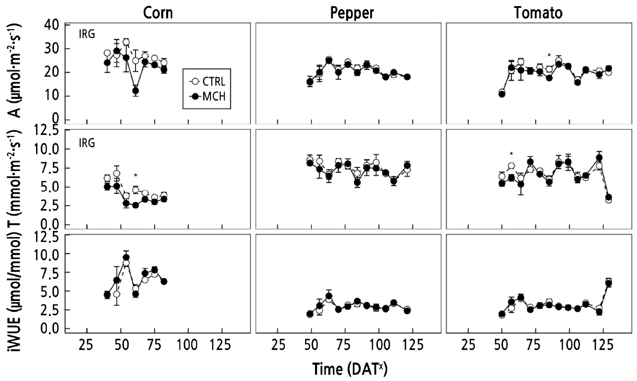
Fig. 2.
Time course responses of leaf physiological characteristics (top/middle/bottom for A, net CO2 assimilation rate/T, transpiration rate/iWUE, instantaneous water use efficiency) for corn (left), peppers (center), and tomatoes (right) under the two different irrigation treatments of surface drip irrigation (SDI) without plastic mulch (white with dashed line, CTRL) and SDI with plastic mulch (black with solid line, MCH). Symbols are the mean responses of four replications, with error bars indicating the ± 1 SEs of the means. Asterisks indicate significant differences of CTRL vs. MCH comparison at each time point at the p < 0.05 level. Overall significant differences at the p < 0.05 level in CTRL vs. MCH comparisons on repeated time course measures are also provided as IRG in the left top corner of each panel if applicable. zDays after transplanting. Corn was directly planted.
Plant Yield Components
For corn, where only harvestable, marketable fruits were collected, plant counts, total FW outcomes, and yields were similar under CTRL and MCH (p > 0.05, Table 3). The marketable yields were 10.3 and 9.81 Mg FW ha-1 for CTRL and MCH, respectively, above the state average of 8.78 Mg FW ha-1 but below the US average of 25.9 Mg FW ha-1.
For peppers, the fruit FW total and total yield were both higher under MCH compared to CTRL (p = 0.049 and 0.049, respectively, Table 3). Although the marketable/unmarketable fruit ratio was not statistically different (p = 0.057), the marketable fruit count and fruit FW were higher in MCH than those in CTRL (p = 0.048 and 0.033, respectively), leading to a significant increase in the marketable yield in the MCH case (p = 0.033). The marketable yields for CTRL and MCH were 22.9 and 33.3 Mg FW ha-1, respectively, both being above the state average of 6.90 Mg FW ha-1. The marketable yield for MCH was even greater than the US average of 29.3 Mg FW ha-1.
Table 3.
Yield components of corn, pepper, and tomato fruits grown under two irrigation treatments – surface drip irrigation (SDI) without plastic mulch (CTRL) and SDI with plastic mulch (MCH) – of the field experiment 2018. The means of each variable are reported with the ± 1 SEs of the means (n = 3)
| Species |
Irrigation treatment |
Plant count (unitless) |
Fruit count total (unitless) |
Fruit count per plant (unitless) |
Fruit FW total (kg FW) |
Fruit FW per plant (kg FW) |
Fruit FW per fruit (g FW) |
Yield (Mg FW ha-1) |
| Cornz | CTRL | 21.3 ± 3.18 ay | - | - | - | - | - | - |
| MCH | 22.0 ± 1.15 a | - | - | - | - | - | - | |
| P-value | 0.853 | - | - | - | - | - | - | |
| Pepper | CTRL | 13.0 ± 0.577 az | 617 ± 42.1 a | 47.7 ± 4.61 a | 27.1 ± 0.81 b | 2.10 ± 0.156 a | 43.3 ± 3.33 a | 26.4 ± 0.79 b |
| MCH | 13.7 ± 0.882 a | 792 ± 81.0 a | 57.6 ± 2.71 a | 37.4 ± 3.59 a | 2.73 ± 0.184 a | 46.7 ± 3.33 a | 36.4 ± 3.49 a | |
| P-value | 0.561 | 0.127 | 0.137 | 0.049*x | 0.058 | 0.518 | 0.049* | |
| Tomato | CTRL | 6.00 ± 1.73 az | 187 ± 29.9 a | 40.5 ± 18.6 a | 13.5 ± 0.19 a | 2.78 ± 0.937 a | 76.7 ± 12.0 a | 29.1 ± 0.42 a |
| MCH | 6.67 ± 0.33 a | 189 ± 53.7 a | 27.6 ± 7.03 a | 17.4 ± 6.42 a | 2.53 ± 0.876 a | 86.7 ± 12.0 a | 37.5 ± 13.8 a | |
| P-value | 0.724 | 0.979 | 0.553 | 0.577 | 0.858 | 0.587 | 0.577 | |
| Species |
Irrigation treatment |
Market ratio (%) |
Market fruit count (unitless) |
Market fruit count per plant (unitless) |
Market fruit FW total (kg FW) |
Market fruit FW per plant (kg FW) |
Market fruit FW per fruit (g FW) |
Market yield (Mg FW ha-1) |
| Cornz | CTRL | - | - | - | 4.80 ± 0.395 a | 0.230 ± 0.020 a | - | 10.3 ± 0.851 a |
| MCH | - | - | - | 4.56 ± 0.673 a | 0.213 ± 0.039 a | - | 9.81 ± 1.450 a | |
| P-value | - | - | - | 0.773 | 0.724 | - | 0.772 | |
| Pepper | CTRL | 79.3 ± 1.76 a | 489 ± 36.0 b | 37.9 ± 4.17 a | 23.5 ± 0.811 b | 1.82 ± 0.142 b | 50.0 ± 0.00 a | 22.9 ± 0.79 b |
| MCH | 87.7 ± 2.85 a | 692 ± 62.8 a | 50.6 ± 2.62 a | 34.2 ± 3.240 a | 2.50 ± 0.184 a | 50.0 ± 0.00 a | 33.3 ± 3.16 a | |
| P-value | 0.057 | 0.048* | 0.062 | 0.033* | 0.042* | 1 | 0.033* | |
| Tomato | CTRL | 23.4 ± 7.27 a | 39.3 ± 6.33 a | 7.26 ± 1.27 a | 4.92 ± 1.19 a | 0.907 ± 0.209 a | 123 ± 13.3 a | 10.6 ± 2.57 a |
| MCH | 22.1 ± 6.83 a | 47.7 ± 24.1 a | 6.90 ± 3.37 a | 5.73 ± 3.02 a | 0.827 ± 0.424 a | 117 ± 3.33 a | 12.3 ± 6.51 a | |
| P-value | 0.906 | 0.754 | 0.924 | 0.814 | 0.873 | 0.653 | 0.814 | |
For tomatoes, no statistical significance was found in the measured matrices, although trends similar to those in the pepper yield data were observed. It is noteworthy that the marketable/unmarketable fruit ratios among the two irrigation treatments were low and not significantly different from each other, ranging from 22.1 to 23.4%. Regarding the marketable yield, 12.3 Mg FW ha-1 in the MCH case was slightly higher than the state average of 12.1 Mg FW ha-1, but this was 87.7% lower than the US average of 100.1 Mg FW ha-1.
Tomato Spotted wilt Virus Damage Assessment
Peppers were not significantly injured by TSWV, as 4.5 and 1.5% of the plants overall were infected in the CTRL and MCH cases, respectively (Table 4). Peppers had a lower incidence of virus infection with MCH (p < 0.001). In contrast, tomatoes had a higher percentage of TSWV damage, as 14.9 and 20.3% of the plants showed virus-like symptoms in the CTRL and MCH treatments, respectively. The resultant dead plants amounted to 16.7 and 9.9% for tomatoes in the CTRL and MCH cases, whereas only 0.5% pepper plants died. For both peppers and tomatoes, all sub-samples of suspected virus-like leaves were found to be TSWV infected, except for one sample from the CTRL tomatoes (Table 4).
Table 4.
Tomato spotted wilt virus (TSWV) diagnosis results of pepper and tomato plants at harvest grown under two irrigation treatments – surface drip irrigation (SDI) without plastic mulch (CTRL) and SDI with plastic mulch (MCH) – of the field experiment 2018. The means of each variable are reported with the ± 1 SEs of the means (n = 3)
| Species |
Irrigation treatment |
Plant count (unitless) |
Virus-like foliage (%) |
Curly foliage (%) |
Dead plant (%) |
TSWV detectionz (%) |
| Pepper | CTRL | 65.3 ± 1.20 ay | 4.59 ± 0.14 a | 34.9 ± 32.6 aw | 0.529 ± 0.529 a | 100 ± 0.00 a |
| MCH | 64.3 ± 1.20 a | 1.56 ± 0.05 b | 2.58 ± 1.02 a | 0.505 ± 0.505 a | 100 ± 0.00 a | |
| P-value | 0.587 | < 0.001***x | 0.377 | 0.975 | 1 | |
| Tomato | CTRL | 30.3 ± 2.19 a | 14.9 ± 5.19 a | 18.2 ± 10.5 a | 16.7 ± 1.29 a | 91.7 ± 8.33 a |
| MCH | 28.3 ± 2.03 a | 20.3 ± 4.33 a | 8.43 ± 4.87 a | 9.95 ± 3.74 a | 100 ± 0.00 a | |
| P-value | 0.539 | 0.444 | 0.614 | 0.164 | 0.373 |
zTwo to four top shoots were sub-sampled from the plants containing virus-like leaves and processed for TSWV detection by qPCR (see Materials and Methods section).
yDifferent alphabetical letters indicate significant differences between treatment groups separated according to Tukey’s HSD post-hoc analysis at the α = 0.05 level.
Crop Evapotranspiration and Water use Efficiency
Average daily and cumulative ETc were slightly lower under MCH compared to CTRL, but the decreases were not statistically significant (p = 0.106, 0.473, and 0.099, respectively for corn, peppers, and tomatoes, Table 2 and Fig. 3 middle panels). For corn, the cumulative ETc outcomes were 478 and 442 mm under CTRL and MCH, respectively. The same trends were found for peppers and tomatoes. The cumulative ETc results were 519 and 506 mm for peppers and 530 and 506 mm for tomatoes under CTRL and MCH, respectively.
Combined with the marketable yield data (Table 3 and Fig. 3, top panels), the differences in ETc between the two treatments (Fig. 3, middle panels) resulted in higher pWUE levels in MCH vs. CTRL for peppers, but not for corn or tomatoes (Fig. 3, bottom panels). The water-use efficiency productivity rates were 2.15 and 2.21 kg FW m-3 water used for corn under CTRL and MCH, respectively (p > 0.05, Fig. 3, bottom left panel). In peppers, the pWUE outcome with the MCH treatment was 6.58, significantly higher than 4.41 kg FW m-3 water used with the CTRL treatment (p < 0.05, Fig. 3, bottom center panel). For tomatoes, pWUE results were 2.01 and 2.43 kg FW m-3 water used under CTRL and MCH, respectively, showing a trend similar to that observed for corn and peppers. However, owing to the large variation in the marketable yield that possibly stemming from TSWV and herbicide drift damage, the difference between CTRL and MCH in tomatoes was not significant (p > 0.05, Fig. 3, bottom right panel).

Fig. 3.
Production characteristics (top/middle/bottom for marketable yield/ETc, crop evapotranspiration/pWUE, water use efficiency of productivity) for corn (left), peppers (center), and tomatoes (right) at harvest under the two different irrigation treatments of surface drip irrigation (SDI) without plastic mulch (white with dashed line, CTRL) and SDI with plastic mulch (black with solid line, MCH). Bars are the mean responses of four replications, with error bars indicating the ± 1 SEs of the means. Different alphabetical letters indicate significant differences between treatment groups separated according to Tukey’s HSD post-hoc analysis at the α = 0.05 level.
Discussion
In the present study, we investigated the feasibility of high-value vegetable production using SDI systems combined with plastic mulch in the semi-arid, windy Texas High Plains. The results demonstrated the utility of plastic mulch to facilitate early crop establishment and to reduce the amount of water required for irrigation. However, contrary to expectations, ETc was not reduced with plastic mulch. Plastic mulch was only effective for increasing pWUE in peppers. Damage from TSWV was identified as a biotic factor that limited the marketable yield of tomatoes, but there was no consistent impact of an irrigation treatment on the incidence of disease in tomatoes or peppers. Although peppers are susceptible to TSWV and some plants here tested positive for infection, the subsequent disease did not significantly impact the yields.
High Winds Presenting Challenges to Vegetable Production in Texas High Plains
Over the growing season, plants were constantly exposed to high winds (Table 1). High winds can have detrimental effects on crop production in many aspects. Micro-environmentally, given that wind speed serves as a primary driver of ET0, high winds can cause a high ET0 outcome, resulting in inevitable water loss from the surfaces of the soil and plants (Paulson, 1991). When combined with high air temperatures and solar radiation, the possible loss of water can be even greater, and this was observed in the present study, where ET0 during the study period was greater than in previous years at the same study site (Colaizzi et al., 2017). Physiologically, high winds can disturb the leaf surface, resulting in the closure of the stomata, which can limit the photosynthetic CO2 uptake and further constrain the production of a crop (Caldwell, 1970). Physically, high winds can mechanically damage the crops, although this type of damage can also be caused by other factors that frequently accompany high winds, such as hail or flooding caused by heavy rain (Gardiner et al., 2016).
Indeed, how to overcome high winds and other adverse weather events has long been an agricultural issue in the Texas High Plains (Colaizzi et al., 2009; Wallace et al., 2012). Nevertheless, it affects row crops to a lesser extent because these crops are usually planted at a high planting density such high winds do not disturb the crops in the rows once the crop canopy is fully closed. In comparison, vegetables are planted with relatively sparse distances between rows to ensure easier access to individual plants for management and harvesting purposes, making individual plants openly exposed to high winds.
Faster Growth and Early Stand Establishment with Plastic Mulch
For all vegetables, faster growth and early establishment were observed under MCH, but the plant growth under MCH was eventually equaled under the CTRL irrigation treatment (Fig. 1). Faster growth and early establishment with plastic mulch has been reported in other studies and is highly correlated with soil or root zone temperatures (Díaz-Pérez, 2010; Bu et al., 2013; Gong et al., 2017; Zhang et al., 2017). In some cases (Ibarra et al., 2001; Yaghi et al., 2013), faster early growth can extend to final yields, but this was not observed in our study. Our results verified increased average daily minimum soil temperatures with increased leaf area and early biomass levels by plastic mulch (Table 2 and Fig. 1). Plastic mulch prevents the escape of long-wave radiation from the soil surface, delaying heat dissipation after sunset overnight. This heat retention effect is more prominent at the early growing stage when the canopy is scarce such that the interception of solar radiation is rare (Dang et al., 2016). Increased soil temperatures promote root growth and expansion, allowing for successful early establishment. This could be a definite advantage for transplants, considering that there is a high risk of encountering weather extremes – high winds, storms with hail, freezing nighttime temperatures – in early spring in the Texas High Plains. Despite the diminishing advantage over time (Fig. 1), having strong crop stands and optimizing conditions for early plant development immediately after transplanting can lower the risk of failure.
Others have accomplished this with the temporary installation of low tunnels (row covers) early in the growing season to optimize environmental conditions for transplant establishment and growth (Lamont, 2005). However, in a climate like that of the Texas High Plains, low tunnels have limited use in the open field due to the very high springtime winds common throughout the region. Rather, a practical solution to the negative effects of high winds could be to increase the planting density to create a canopy sooner in the early growing season or to place windbreaks on the edges of the plots. Also, building protective structures for plants, such as high tunnels to cover an entire cropping system, may be an option (Lamont, 2005).
Attainable Marketable Yields in Corn, Superior Marketable Yields in Peppers and Losses of Marketable Yields in Tomatoes by TSWV
The effects of plastic mulch on yield components were observed exclusively in peppers and not in corn or tomatoes (Table 3). For corn, the marketable yields both from CTRL and MCH exceeded the state average, indicating that fresh market sweet corn could be a viable option for high-value crop production. With plastic mulch, there was a 14.8% increase in the marketable yield for peppers. Lower incidence rates of virus infection were observed as well with plastic mulch in peppers (Table 4). For tomatoes, the percentage of marketable fruits was very low, ≈20%, in both irrigation treatments (Table 3 and Fig. 3), clearly demonstrating the high risk associated with open-field production of tomatoes in the Texas High Plains region. This significant fresh marketable yield loss was largely due to damage from TSWV (Table 4). Near harvest time, approximately ≈20% of the plants exhibited typical foliar symptoms of tomato spotted wilt and ≈10–17% of the plants had already succumbed to the disease and had died. Also, we observed that approximately ≈8–18% of the plants exhibited severe leaf curl, likely due to insects, herbicide drift, or wind damage. All of these abiotic/biotic sources of stress resulted in tomato yields below the state average. Management practices to overcome these challenges would be essential for open-field tomato production (Wallace et al., 2011).
At the outset of this study, a significant increase in pWUE for all vegetables was expected with plastic mulch owing to the semi-arid environment in which the study would be conducted. However, this result was observed only with peppers and not with corn or tomatoes. Indeed, the amount of water applied was reduced by 7.4%, and the amount of water used – ETc – was slightly reduced with plastic mulch for all vegetables, but the reductions were not significant (p = 0.106, 0.473, and 0.099 for corn, peppers, and tomatoes, respectively). Similar findings were reported in which the authors found that the use of plastic mulch did not reduce total water use, as measured by ETc, for spring maize in a semi-arid dryland region in China (Li et al., 2008). Instead, plastic mulch changed the proportion of evaporation to transpiration, and these two factors together comprise the ETc of plants. Water loss from transpiration was increased and evaporation was decreased with plastic mulch. However, in our study, as the canopy expanded and shaded the soil surface, evaporation was reduced and became less important in relation to crop water use, as most water loss took place on the leaf surface through transpiration. For this reason, the effects of plastic mulch on crop water use faded as crop growth progressed toward the full canopy stage. In line with this finding, other research reported that the effects of plastic mulch on increased soil temperatures are reduced as the canopy expands (Zhao et al., 2012). This was also observed here.
The diminishing plastic mulch effects on crop water use may explain the differences in the pWUE responses among species in the study. Peppers showed a significant increase in pWUE under MCH compared to CTRL, whereas corn and tomatoes showed no differences (Fig. 3). Peppers have relatively low leaf coverage of the soil surface compared to corn and tomatoes. When the leaf area data are combined with the plant count data (Fig. 1 and Table 3, respectively), corn and tomatoes at harvest had around 1.5- and 3-fold greater canopy areas that covered the soil surface compared to that of peppers. Thus, with less soil space exposed, even under CTRL, the comparative advantage of mulching on evaporation was likely reduced for corn and tomatoes.
Species-specific Summary of the Study
For corn, given that most regional growers are already familiar with field corn and have general knowledge of production, sweet corn could be an attractive crop choice when using SDI systems. However, the use of plastic mulch with sweet corn would not be recommended. Despite the fact that mulching resulted in faster establishment of crop stands, which is always beneficial in the Texas High Plains due to the harsh environmental conditions in early spring, mulching did not result in increased yields. The yield gap between the state and the national averages is about three-fold, meaning that sweet corn cultivation could be a good selection, as gradual yield increases over the years are achieved.
For peppers, due to their high market value and high productivity, we identify this crop as the most viable option compared to sweet corn and tomatoes for production with SDI systems. Furthermore, with plastic mulch, maximum yields and WUE outcomes can be achieved.
For tomatoes in open-field conditions, it could be difficult to achieve an economically viable crop, even when using a SDI system, due to the potential for extreme losses to both biotic and abiotic stressors. Each year, open-field production of tomatoes in the High Plains will be exposed toe to high winds, hail, and threats from TSWV. Accordingly, protective cropping systems such as high tunnels would be required to produce maximum yields of high-quality, marketable tomatoes dependably.
