Introduction

Ziziphi spinosae semen (ZSS) is one of the most widely used medicinal herbs in traditional Chinese medicine (Chen et al. 2011). ZSS exhibits therapeutic effects in the management of insomnia, palpitations, anxiety, sweating, and memory problems. It also supports the health of the heart and liver while providing a calming effect on the mind (Xie 1996; Fang et al. 2010). In China, ZSS is a common component of at least 67% of traditional Chinese medicine prescriptions used to treat insomnia, depression, and anxiety (Yeung et al. 2012). ZSS is characterized by very low oral toxicity. Despite its potent effects, it remains relatively safe for long-term use and is considered safe for use in children (Zhang et al. 2009). Owing to its high value and popularity, its price has increased, and the use of substitutes has become increasingly common as sellers seek to maximize profit (Sun et al. 2014; Xia et al. 2023). In Korea, ZSS is imported exclusively, resulting in a heightened risk of adulteration. Ziziphi mauritianae semen (ZMS), which is morphologically similar and difficult to distinguish, is widely used as an adulterant (Zhang et al. 2016; Yan et al. 2020; Chen et al. 2024). However, due to insufficient verification of the efficacy and potential side effects of ZMS, its distribution has been completely prohibited in Korea. The primary constituents of ZSS and ZMS differ, resulting in distinct therapeutic effects (Yan et al. 2020). This discrepancy poses a potential threat to consumer health, highlighting the urgent need for an accurate differentiation between ZSS and ZMS (Li et al. 2023).

Studies have been conducted to distinguish between ZSS and ZMS using morphological and chemical methods (Yan et al. 2020; Xia et al. 2023). Typically, ZSS has a flattened oval shape with a longitudinal ridge at the center and a smooth, purplish-brown glossy surface, whereas ZMS is generally wider and flatter without a central groove and features a clay-like color with irregular dark-brown markings. However, these differences are not easily discernible by the public (Xia et al. 2023). When only simple RGB- and texture-based computer vision techniques are applied to the original data, distinguishing the two samples remains challenging, with classification accuracy limited to approximately 70–80% (Chen et al. 2024). RAPD-PCR has been employed to identify genetic markers specific to ZSS; however, this method is destructive and prone to variability, which can compromise its reproducibility (Xia et al. 2023). Similarly, chemical ultra-performance liquid chromatography quadrupole time-of-flight mass spectrometry (UPLC-Q-TOF/MS) has demonstrated a clear differentiation between the two species based on key metabolites (Yan et al. 2020); however, it requires expensive equipment, complex procedures, and specialized expertise. These limitations underscore the need for more efficient, nondestructive, and reproducible methods to reliably differentiate between ZSS and ZMS.

These methods are time-consuming, rely heavily on experience, and are typically destructive, making them impractical for application to all seeds in distribution (Yang et al. 2011). In particular, ZMS is typically illicitly distributed not as a complete substitute but rather through partial admixture with ZSS, making it difficult to ensure overall product quality by testing only a limited number of representative samples. In addition, the appearance of ZSS varies depending on its five geographical origins (Zhao et al. 2024). This implies that there is considerable variation in color, even within the ZSS itself, indicating that distinguishing ZSS from ZMS based solely on color is unreliable.

This study proposes the use of hyperspectral imaging (HSI) to address the limitations of existing methods. HSI is a non-contact, non-destructive technique that can be performed directly in the field (Chlebda et al. 2017), providing rapid and accurate information on both the internal and external properties of seeds. Moreover, HSI-based models are powerful analytical tools with a high potential for identifying and differentiating features on sample surfaces (Taghizadeh et al. 2011). This technology has been validated to identify a wide range of crops, such as grains, fruits, and vegetables, demonstrating its effectiveness in distinguishing among various seed types (Guo et al. 2017; Qiu et al. 2018; Zhu et al. 2019; Li et al. 2021).

Hyperspectral data collects images across various wavelengths and stores them in the form of a data cube, enabling the acquisition of spectral information beyond the visible spectrum (Velasco-Forero and Manian 2009). This enables the detection of subtle spectral differences related to the chemical composition, facilitating the precise differentiation of varieties and origins (Wu et al. 2021; Xu et al. 2022). Additionally, HSI technology can simultaneously analyze a large number of individual seeds, making it highly suitable for large-scale seed purity assessments (Wu et al. 2021). For instance, HSI achieved 98.36% accuracy in classifying corn seeds (Li et al. 2024), 95.19% accuracy in identifying soybean varieties (Wang et al. 2022), and 95–99.57% accuracy in distinguishing rice, oat, wheat, and cotton seeds (Wu et al. 2021).

Preprocessing of spectral data is crucial for minimizing the unnecessary effects of measurement conditions and emphasizing useful features (Velasco-Forero and Manian 2009). This process typically involves normalization, derivation, and smoothing. In addition, because hyperspectral images contain vast amounts of high-dimensional data, appropriate artificial intelligence models are necessary to efficiently interpret spectral information (Makantasis et al. 2018). Without such models, there is a risk of insufficient utilization of spectral data or reduced accuracy. AutoGluon, an open-source automated machine learning (AutoML) library developed by Amazon, automates the entire machine learning model development process to achieve high performance in various tasks, such as image classification and object detection (Erickson et al. 2020; Shi et al. 2021). In this study, AutoGluon was employed to simplify the complex machine-learning workflow and select the optimal combination of preprocessing methods and corresponding model.

This study 1) developed a rapid, non-destructive classification method for distinguishing between ZSS and ZMS by integrating HSI with AutoGluon, 2) built a high-performance classification model through automated optimization and ensemble modeling, and 3) established a novel analytical approach for the authentication and quality control of medicinal herbs by identifying the spectral differences between ZSS and ZMS. These contributions are expected to significantly advance the safety and standardization of herbal medicines.

Materials and Methods

Collecting samples

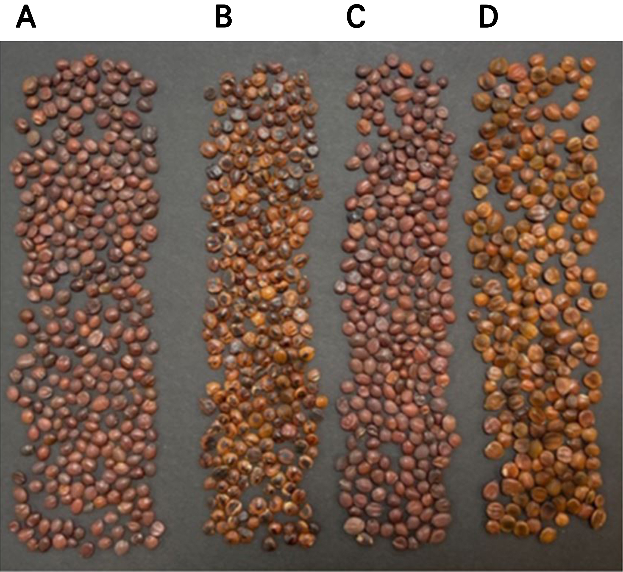
The ZSS and ZMS samples used in this study were provided by the Quality Certification Center of the National Institute for Korean Medicine Development. Representative images of the ZSS and ZMS samples collected from different origins are shown in Fig. 1. Although all samples were provided by a single institution, they were collected from four different geographical origins, and therefore represent a range of origin-related variation. For both ZSS and ZMS, 25 samples were randomly collected from each of four different origins, yielding 100 samples per group and a total of 200 samples.

Fig. 1.

A and C represent Ziziphi spinosae semen (ZSS) collected from different sources, while B and D represent Ziziphi mauritianae semen (ZMS) from distinct sources.

Description of hyperspectral equipment

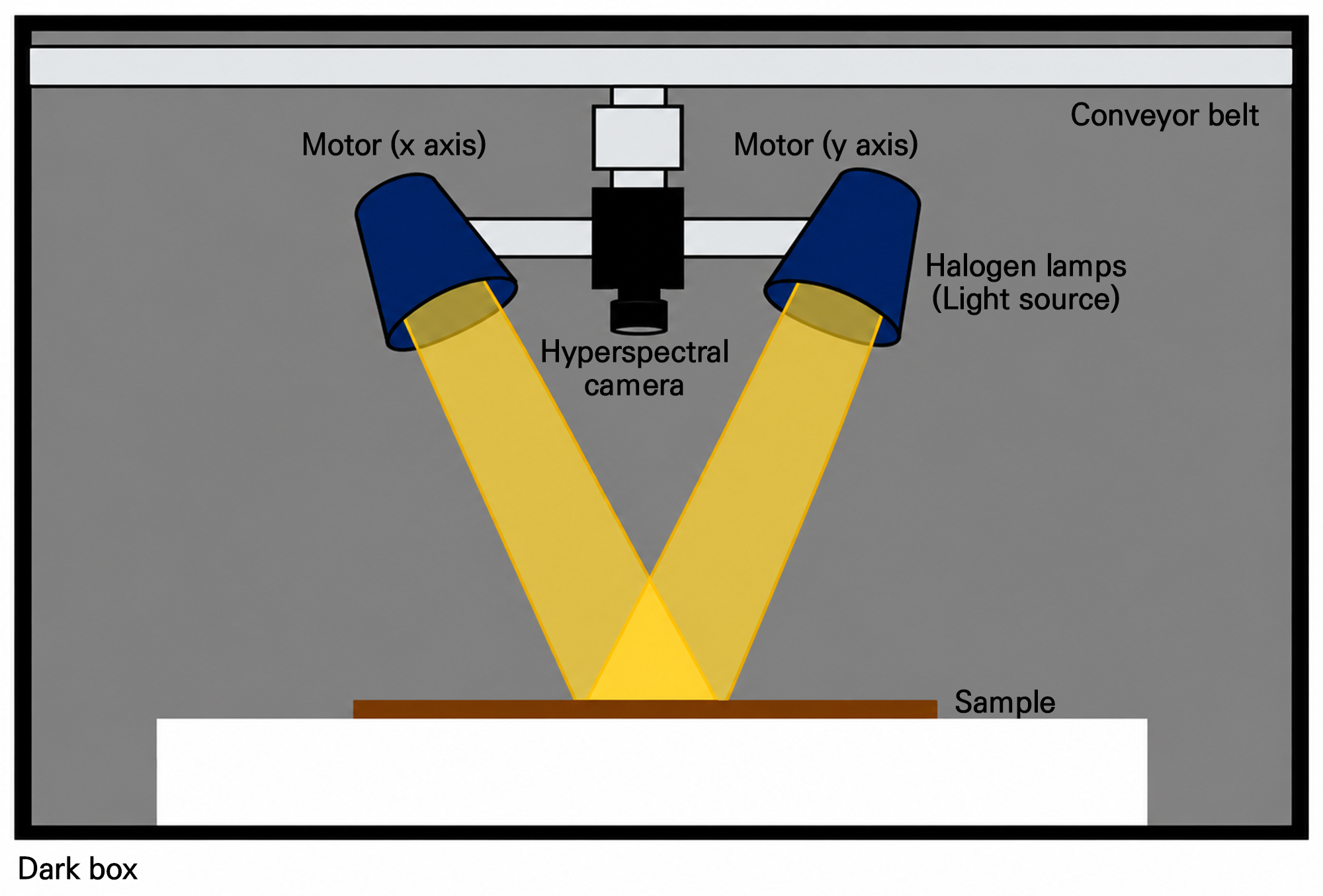
The hyperspectral reflectance images of the samples were collected using the HSI system shown in Fig. 2. Imaging was conducted inside a light-blocked chamber equipped with eight 20 W halogen lamps and a hyperspectral camera. A MicroHSI 410 SHARK camera (Corning Inc., Corning, NY, USA) was used. During image acquisition, the system employed a line scan method in which the camera remained fixed along the y-axis and moved horizontally along the x-axis at 100 mm/s, as configured using desktop software. For spectral data collection, labeled seeds were arranged in order on a black matte plate that prevented light reflection. Hyperspectral images were captured using an HSI camera with 150 spectral bands spanning wavelengths from 400 nm to 1,000 nm.

Fig. 2.

Hyperspectral imaging system.

Preparation of extract and UPLC analysis

Dried samples were subjected to 75% ethanol (100 mg per 1 mL) extraction at 300 W under sonication (UCP-10; Lab-Companion, Republic of Korea) at 50°C for 20 min. Extracts were centrifuged at 13,000 rpm for 5 min at 4°C and filtered through a 0.22 µm membrane filter and used for UPLC analysis.

For quantification of the target compounds, jujuboside A was purchased from Samsung Industrial Company, LTD. It was dissolved in DMSO to a concentration of 1 mg/ml. Sample and standard analyses were conducted using an ultra-high-performance liquid chromatograph (Agilent 1260 series) equipped with two pumps, a column oven, an autosampler, and a diode array detector. A 20  µL sample was loaded onto a YMC-Triart C18 ODS column (100 × 2.0 mm I.D., 1.9 µm particle size, 12 nm pore size; YMC Co., Ltd., Japan) set at 30°C. A gradient elution system using two solvents was employed: water containing 0.2% formic acid (A) and acetonitrile containing 0.2% formic acid (B). The initial solvent ratio of B was set at 75% and maintained for 4 min, then increased to 90% B over 10 min to facilitate gradient elution. The solvent system was subsequently reequilibrated from 10.5 to 13 min under 75% B conditions.

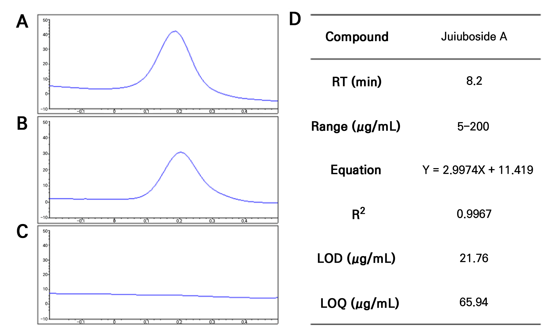
Jujuboside A was used as a marker to classify ZSS and ZMS. A range of concentrations (5–200 µg per 1 mL) of jujuboside A was prepared to construct a calibration curve. The presence of jujuboside A indicated ZSS, whereas its absence indicated ZMS (Kim et al. 2014).

Spectral data collection and preprocessing

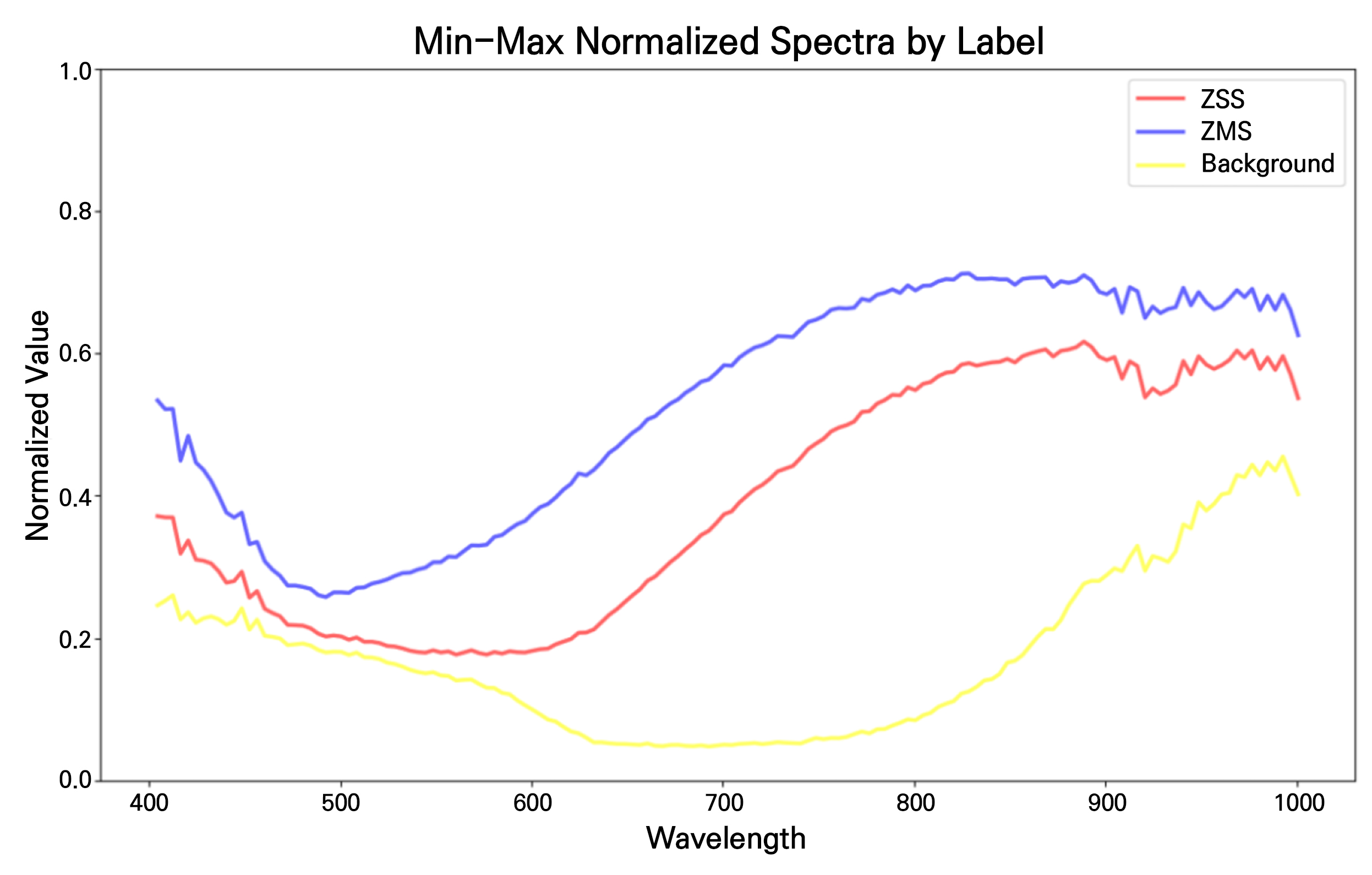
Spectral data were extracted from 100 samples from each class: ZSS, ZMS, and background. For each ZSS and ZMS seed, 64 pixels were extracted from the central region using an 8 × 8 square grid to minimize background influence. Background pixels were randomly selected from multiple locations across the image to ensure representative sampling. Each extracted pixel contained reflectance information from 150 spectral bands. The mean min–max-normalized spectra of ZSS, ZMS, and background are shown in Fig. 3 to illustrate the overall spectral characteristics of the three classes before additional preprocessing. Based on the UPLC results, six ZSS samples and 25 ZMS samples were excluded. The final dataset consisted of 94 ZSS samples, 75 ZMS samples, and 100 background samples.

Fig. 3.

Averaged reflectance spectra of ZSS, ZMS, and background classes following min–max normalization.

Spectral data are inevitably influenced by a variety of factors; therefore, spectral preprocessing is employed to enhance their reliability and usefulness (Esquerre et al. 2012).

All pixel values were normalized using min–max scaling as follows:

xscaled=x-xminxmax-xmin

where xscaled denotes the normalized data value, x the original data value, xmax the maximum value of the feature, and xmin the minimum value of the feature.

Various preprocessing methods were applied to the spectral data, either individually or in combination. These methods include the standard normal variate (SNV) (1), first (2) and second derivatives (3), and Savitzky–Golay smoothing (4). The mathematical expressions for each method are expressed in Eqs. (1), (2), (3), (4).

Here, x denotes the original spectrum, x¯ and 𝜎 denote the mean and standard deviation of the spectrum, respectively, while h indicates the interval in the independent variable. In the Savitzky–Golay filter (Eq. (4)), yı^ represents the filtered output at the i-th position, yi+j denotes the input value at position (i+j), cj represents the filter coefficients, and m determines the filter order and window size.

To obtain reliable analytical results, it is essential to minimize interfering variations through appropriate mathematical preprocessing. Accordingly, multiple preprocessing methods and their combinations were systematically evaluated, and the combination that achieved the best cross-validated classification performance was selected for the final model.

SNV normalization was applied to correct variations in spectral intensity caused by external factors, such as surface texture, thickness, and lighting conditions, rather than the chemical composition of the sample. This correction reduces irrelevant intensity differences and emphasizes the meaningful spectral characteristics associated with the sample’s intrinsic properties (Barnes et al. 1989).

The first derivative was used to eliminate baseline offsets and highlight slope changes in the spectra, thereby allowing fine absorption features to be separated more distinctly. This enhances the interpretability of the spectra, particularly when the peaks are closely located or partially overlapping (Hopkins 2001; Davies 2007; Rinnan et al. 2009).

The second derivative emphasizes the curvature of the spectral signal, improving the resolution of peak shapes and locations. Additionally, it removes linear trends from the baseline, helping to isolate meaningful spectral information from background variations (Davies 2007).

Savitzky–Golay smoothing was employed to reduce high-frequency noise by fitting the local segments of the spectrum with smooth polynomial curves. This technique softens the data while preserving critical spectral structures, such as absorption peaks, thereby effectively balancing noise suppression and signal retention (Savitzky and Golay 1964; Davies 2007).

Classification model

This study was conducted in a Python 3.8 environment, utilizing the Pandas, NumPy, Scikit-learn, Matplotlib, and AutoGluon libraries for data analysis and model training. To optimize the classification performance, various preprocessing methods and their combinations were applied to the dataset to identify the most effective approach for each dataset and ultimately select the preprocessing combination and model that achieved the highest overall accuracy. However, manually configuring the models and tuning the hyperparameters for each preprocessing variation is a highly time- and resource-intensive process, which makes it inefficient for practical applications.

Therefore, to address this inefficiency and identify the optimal model systematically and rapidly, AutoGluon was employed. AutoGluon automates model training, hyperparameter optimization, and performance evaluation across a range of machine learning algorithms, thereby minimizing the time required and facilitating the efficient selection of the most appropriate model for dataset characteristics (Erickson et al. 2020).

The dataset was split using 5-fold GroupKFold cross-validation, with folds defined at the level of the physical seed rather than the individual pixel: all 64 pixel spectra belonging to a given seed were assigned entirely to either the training or the held-out test partition within each fold, preventing pixel-level data leakage that would otherwise inflate accuracy. Within each fold, min-max normalization and all spectral preprocessing steps were fit using only that fold’s training partition and then applied to the corresponding test partition. Several predefined preprocessing schemes were evaluated under the same cross-validation framework. The preprocessing scheme that achieved the highest mean accuracy with the lowest standard deviation was selected for the final model.

In this study, the core module of AutoGluon, the TabularPredictor, was employed to automate the training and optimization processes. The AutoGluon-based modeling workflow proceeded as follows. First, the preprocessed dataset, containing spectral features and corresponding class labels, was supplied to the TabularPredictor.fit() function. AutoGluon internally trains multiple machine learning algorithms in parallel, including Random Forest, LightGBM, and CatBoost. To improve the performance, it automatically constructs a stacked ensembling architecture that combines the predictions of individual base models. Model performance was then evaluated through internal validation, and the best-performing model was automatically selected.

To identify which wavelengths contributed most to classification, permutation-based feature importance was computed using AutoGluon’s built-in predictor.feature_importance() function. For each wavelength, values in the held-out test set were randomly shuffled to nullify the information carried by that feature, and the resulting drop in accuracy was recorded as its importance score; a larger drop indicates greater reliance on that wavelength. This procedure was repeated independently for each of the five GroupKFold folds, and the resulting importance scores were averaged.

Thus, the AutoGluon framework offers a distinct advantage by adopting a stacked model-ensembling strategy rather than relying solely on individual models or hyperparameter optimization, thereby maximizing the overall model performance.

Correlation coefficient

To evaluate the wavelength-specific association between spectral features and species identity, point-biserial correlation coefficients were calculated at each wavelength using preprocessed spectra. Each sample was assigned a numerically coded species label (ZSS = 1 and ZMS = 2), and the spectra were subjected to the same preprocessing procedure used for the classification model. The correlation coefficient was defined as follows:

r=∑i=1nxi-x¯yi-y¯∑i=1nxi-x¯2∑i=1nyi-y¯2

where xi denotes the preprocessed spectral value of the i-th sample at wavelength λ, and yi denotes the numerically coded species label of the same sample. The terms x¯ and y¯ represent the mean preprocessed spectral value and mean coded label across all samples, respectively.

In this context, r represents the point-biserial correlation between a continuous spectral variable and a binary species label, which is mathematically equivalent to Pearson’s correlation coefficient. A larger absolute value of r indicates a stronger univariate association between the spectral feature at a given wavelength and species identity. Because first-derivative preprocessing was applied, wavelength-specific associations were primarily interpreted based on the absolute value of r, rather than as direct differences in raw reflectance intensity. The analysis was performed using the final UPLC-verified dataset comprising 94 ZSS and 75 ZMS samples. Because r is computed from the pooled set of all 169 individual samples and their associated labels, rather than from paired comparisons between individual ZSS and ZMS samples, this approach does not require the two groups to be of equal size.

Evaluation of machine learning models

We used a performance evaluation metric to assess the predictive accuracy of our model. The utilization of multiple evaluation metrics enabled a comprehensive assessment of model performance from various perspectives.

The confusion matrix is a widely used visual tool in machine learning for evaluating the performance of classification models (An et al. 2024). This matrix compares the predicted outcomes of the model with the actual labels and provides a quantitative representation of prediction accuracy (Erickson et al. 2020). The rows of the matrix correspond to the actual classes, and the columns represent the predicted classes. This enabled a systematic analysis of the predictive performance of the model. We employed a classification model with three classes, which resulted in a 3×3 confusion matrix containing nine elements. Each element in the matrix represents a specific combination of the actual and predicted classes. This enabled the evaluation of the model’s accuracy in predicting each class and the identification of misclassified instances for further analysis.

Accuracy is a key performance metric derived from the confusion matrix and represents the proportion of correct predictions made by the model. This value was calculated using the following formula:

Accuracy = Number of correctly classified samples Total Number of Samples

A higher accuracy value indicated better overall predictive performance of the model. This metric is relatively simple to compute, has low complexity, and is easily applicable to multiclass and multilabel problems (Bochkovskiy et al. 2020). In this study, a multiclass classification task was conducted (ZSS, ZMS, and background), and performance evaluation was based on a confusion matrix. Here, a true positive (TP) refers to cases in which a specific class (e.g., ZSS) is correctly predicted as ZSS, whereas a true negative (TN) refers to cases in which other classes (e.g., ZMS or background) are correctly predicted as not ZSS.

Balanced accuracy is calculated as the average recall and enables fair evaluation of the model performance, even on datasets with imbalanced class distributions. It is particularly effective in mitigating bias when a dominant class skews the overall accuracy because it evenly reflects the prediction performance across all classes (García et al. 2009).

The Matthews correlation coefficient (MCC) is a comprehensive metric that considers all elements of the confusion matrix to assess the correlation between predicted and actual labels. It is particularly useful for evaluating the overall prediction quality in cases of severe class imbalance, allowing for a more accurate assessment of classification performance that simple accuracy cannot capture (Boughorbel et al. 2017).

Model application

To analyze and visualize the prediction results of the model, a post-processing procedure was implemented that included binarization, contour detection, instance segmentation, label analysis, and color mapping, ultimately culminating in a visual representation of the classification outcomes. For visualization, the predicted labels were first converted into an integer format, and Labels 1 and 2 were considered objects to generate a binary foreground mask. Because a simple connected-component contour search merges physically adjacent or overlapping seeds into a single object, pooling pixels from different seeds into one majority-vote decision, contour detection was replaced with a watershed-based instance segmentation procedure. A Euclidean distance transform was computed on the binary mask, and local maxima of the distance transform (identified with peak_local_max) were used as seed markers for the watershed algorithm, so that adjacent or lightly overlapping seeds were separated into distinct instances prior to labeling. Pixel values within each resulting instance were retrieved, and their label distributions were analyzed using NumPy’s unique function. The label exhibiting the highest frequency within each instance was designated as the representative (majority-vote) label, thereby enabling object-level classification, and the proportion of votes for the winning label (vote margin) was calculated to assess the classification confidence for each object. Finally, color mapping was applied to each object according to the assigned labels: ZSS was rendered in red, ZMS in blue, and the background in black, thus distinguishing objects from the background and facilitating an intuitive evaluation of the classification performance of the model.

Results

UPLC

After collecting the HSI data, the samples were identified using UPLC to increase the reliability of the experiment. Only those verified as ZSS and ZMS by UPLC were used as training data. Considering that UPLC is a destructive analytical method, it was intentionally performed after nondestructive HSI.

As shown in Fig. 4A, jujuboside A was detected at 8.2 min. Its presence varied depending on the sample species. Jujuboside A was not detected in any of the ZMS samples examined, including the darkest specimens, supporting its use as a marker compound specific to ZSS. Additionally, jujuboside A content differed among samples within the ZSS. During UPLC analysis, Sample 65, which was initially classified as ZSS, was identified as ZMS. Additionally, Samples 3, 17, 72, 78, and 99 did not exceed the threshold (0.03% of jujuboside A), indicating low reliability (Kim et al. 2014). Excluding these samples (n = 94), the average jujuboside A content was 0.19 ± 0.10%, with a high variation observed among samples ranging from 0.04% to 0.61%. Consequently, to ensure more accurate classification, these six samples were excluded from the training dataset.

Fig. 4.

UPLC chromatogram of (A) jujuboside A (100 ppm), (B) ZSS sample, and (C) ZMS sample. (D) Linearity, linear ranges, LOD, and LOQ of the calibration curve of jujuboside A for quantification. LOD, limit of detection; LOQ, limit of quantification.

Results of model development

Model selection and spectral preprocessing were re-evaluated using 5-fold GroupKFold cross-validation, with folds defined at the physical-seed level to prevent pixel-level data leakage. Among the preprocessing schemes evaluated, the combination of Savitzky–Golay smoothing, SNV, and first-order derivative preprocessing achieved the highest mean accuracy with low fold-to-fold variability and was therefore selected as the final preprocessing method.

AutoGluon automatically trained and evaluated multiple machine-learning models and constructed a weighted ensemble from the predictions of the candidate base models. The final model selected by AutoGluon was WeightedEnsemble_L2, which assigned 100% of its weight to LightGBMXT. Therefore, although AutoGluon retained the weighted-ensemble structure, the final predictions were effectively generated by the LightGBMXT model.

Across the five GroupKFold test folds, the final model achieved a mean pixel-level accuracy of 98.40% ± 0.91%, a balanced accuracy of 98.21% ± 1.00%, and an MCC of 0.976 ± 0.015. The fold-level accuracies were 97.05%, 98.58%, 99.51%, 98.09%, and 98.76%, respectively. These results were obtained using the final dataset comprising 94 UPLC-verified ZSS seeds, 75 ZMS seeds, and 100 background samples. Overall, the results indicate that the selected preprocessing and AutoGluon-based model provided consistently high classification performance under seed-grouped cross-validation.

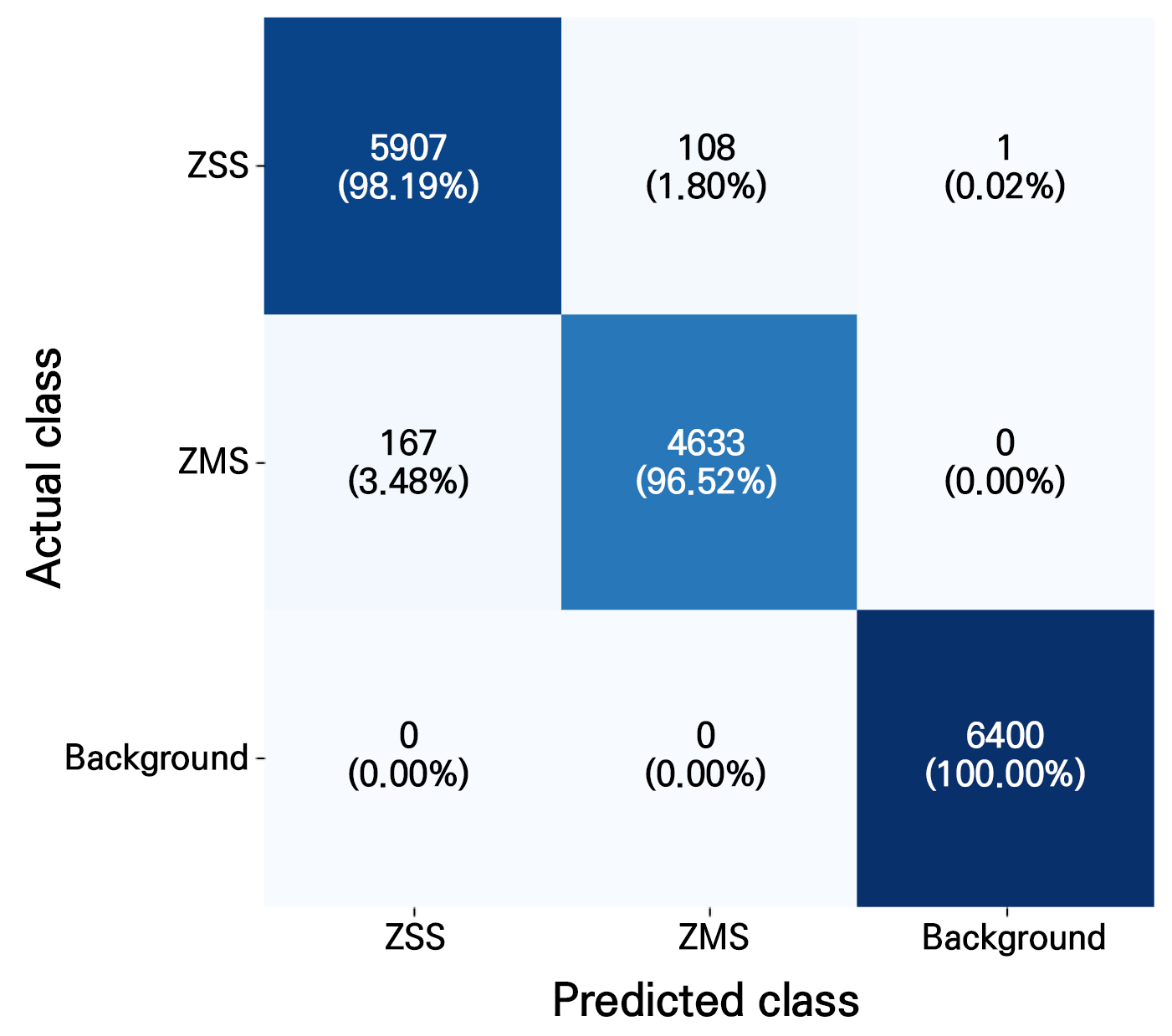
Figure 5 presents the confusion matrix obtained by aggregating the pixel-level predictions from all five GroupKFold folds. Misclassification remained low and asymmetric: 1.80% of ZSS pixels (108/6,016) were misclassified as ZMS, and 3.48% of ZMS pixels (167/4,800) were misclassified as ZSS, confirming the effectiveness of the proposed model under cross-validation.

Fig. 5.

Aggregated pixel-level confusion matrix obtained from the five GroupKFold test folds. Rows indicate the actual classes, and columns indicate the predicted classes. Each cell presents the number and row-wise percentage of pixels assigned to the corresponding class.

To identify the wavelength-related features that contributed most to classification, permutation-based feature importance was calculated using AutoGluon’s built-in predictor.feature_importance() function. For each feature, its values in the held-out test set were randomly permuted, and the resulting decrease in classification accuracy was used as the importance score. A larger decrease indicated a greater relative contribution of that feature to model prediction. This procedure was performed independently for each of the five GroupKFold folds, and the resulting importance scores were averaged across folds.

As shown in Fig. 6, 628.66 nm exhibited the highest mean permutation importance among the evaluated features, with a value of 0.0121, followed by 644.66, 596.64, 672.68, and 632.66 nm. All of the top 10 wavelengths were located within the 596–677 nm range, and 628.66 nm ranked first in three of the five folds. Because the model inputs underwent Savitzky–Golay smoothing, SNV, and first-derivative preprocessing, these importance values reflect the contribution of local preprocessed spectral features around the corresponding wavelengths rather than raw reflectance intensity alone. Overall, the results indicate that the model relied on a cluster of adjacent wavelengths in the visible orange–red region(596–677 nm) rather than on a single wavelength.

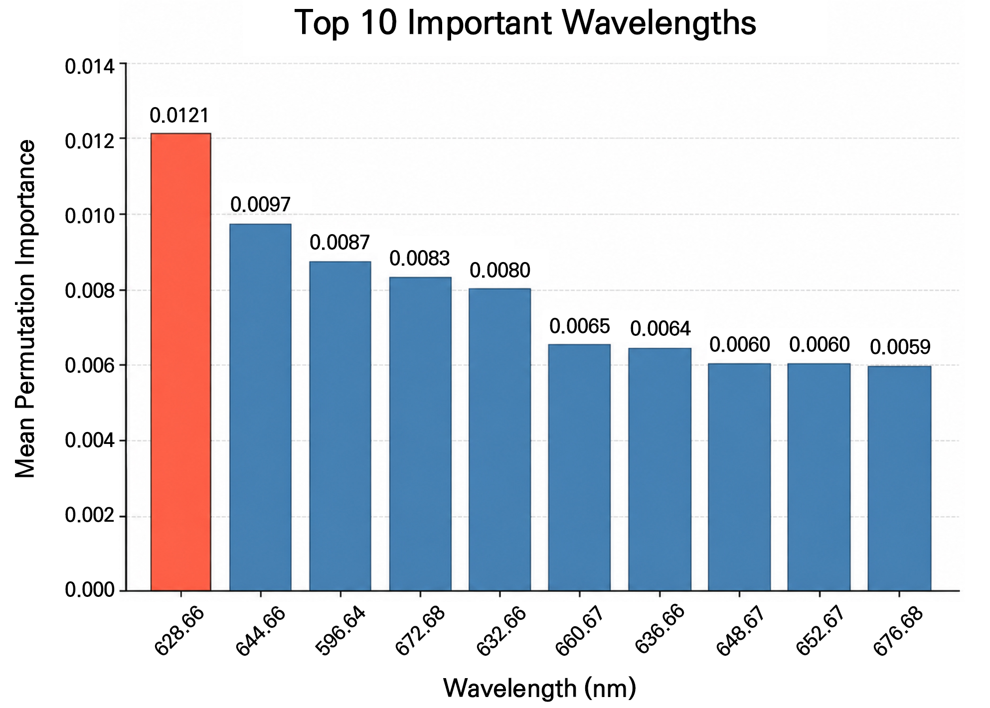
Fig. 6.

Top 10 wavelengths ranked by mean permutation-based feature importance across the five GroupKFold folds. Importance was calculated as the decrease in classification accuracy after randomly permuting each wavelength feature in the held-out test set. The wavelength with the highest mean importance is highlighted in tomato red, while the remaining wavelengths are shown in steel blue. Values above the bars indicate the mean importance scores.

Correlation coefficient analysis

Point-biserial correlation coefficients were calculated at each wavelength using spectra processed with the same Savitzky–Golay smoothing, SNV, and first-derivative transformation selected for the final classification model. High positive correlations were observed across the 600–700 nm region (Fig. 7), with a maximum correlation coefficient of approximately 0.84 near 600 nm, followed by a gradual decrease toward 700 nm. Because the analysis was based on first-derivative spectra, this result does not indicate that one species directly exhibited higher raw reflectance than the other. Instead, it indicates that the local spectral slopes and patterns within this wavelength region differed systematically between ZSS and ZMS.

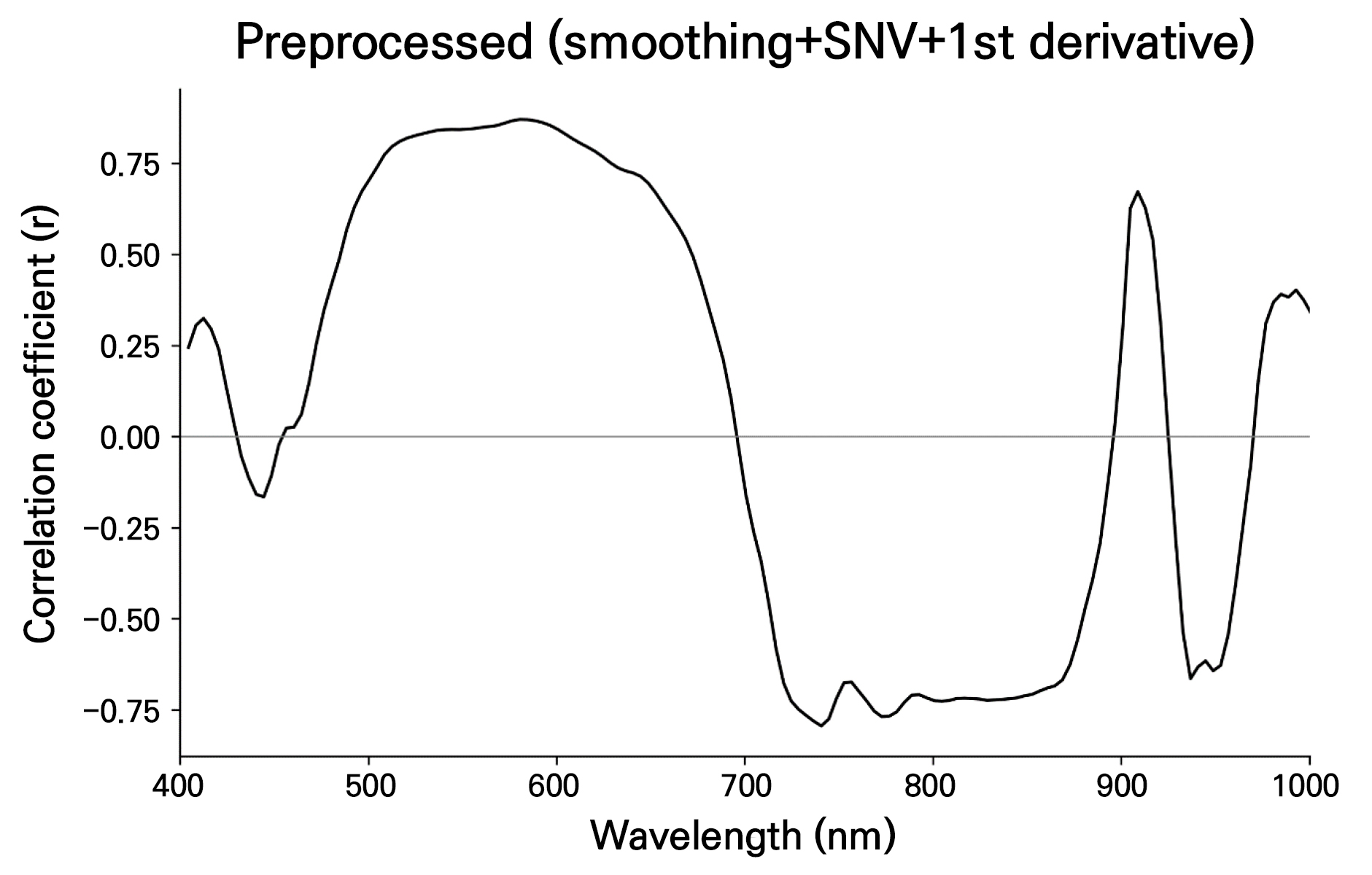
Fig. 7.

Point-biserial correlation coefficients between the preprocessed spectral values and species labels across wavelengths. Spectra were processed using Savitzky–Golay smoothing, SNV, and first-derivative transformation. Positive and negative values indicate the direction of the association, while larger absolute values indicate stronger wavelength-specific associations between the spectral features and species identity.

The broadly elevated correlations across 600–700 nm suggest that this visible spectral region contains substantial information for distinguishing the two species (Sharabian et al. 2014; Tang et al. 2022). However, high absolute correlation coefficients were also observed in other visible and near-infrared regions, and the direction of the association varied with wavelength. Consistent with the 600–700 nm correlation pattern, the permutation importance analysis showed that the classification model relied mainly on wavelengths within this region (Fig. 6). However, univariate correlation alone has limitations in identifying discriminative features (Janse et al. 2021; Xu et al. 2021), and high absolute correlations were also observed in other regions. Therefore, full-spectrum input may provide supplementary information and improve robustness against sample variability (Grewal et al. 2023).

Model application

The pixel-level predictions from the five GroupKFold test folds were aggregated by majority voting to evaluate classification performance at the individual-seed level. Each of the 169 ZSS and ZMS seeds was included in a held-out test fold exactly once. Three seeds were misclassified: two ZMS seeds were classified as ZSS, and one ZSS seed was classified as ZMS. The corresponding recalls were 0.989 for ZSS and 0.973 for ZMS, indicating that misclassification occurred in both directions but was slightly more frequent for ZMS.

The two ZMS seeds misclassified as ZSS exhibited lower raw reflectance than correctly classified ZMS seeds (Fig. 8A). To further examine the position of the misclassified samples in the spectral feature space, PCA was performed using the preprocessed seed-level spectra. Although the ZSS and ZMS samples were generally separated, the misclassified seeds were located near the boundary between the two clusters (Fig. 8B). The mean distance of the misclassified ZMS seeds from the ZMS cluster centroid was 164.9, compared with 75.4 for correctly classified ZMS seeds. In addition, the mean majority-vote margin of the misclassified seeds was 0.729, which was lower than that of correctly classified seeds (0.985), and two of the three misclassified seeds had vote margins below 0.7. These findings show that the misclassified seeds exhibited lower prediction consensus and occupied borderline positions in the preprocessed spectral feature space.

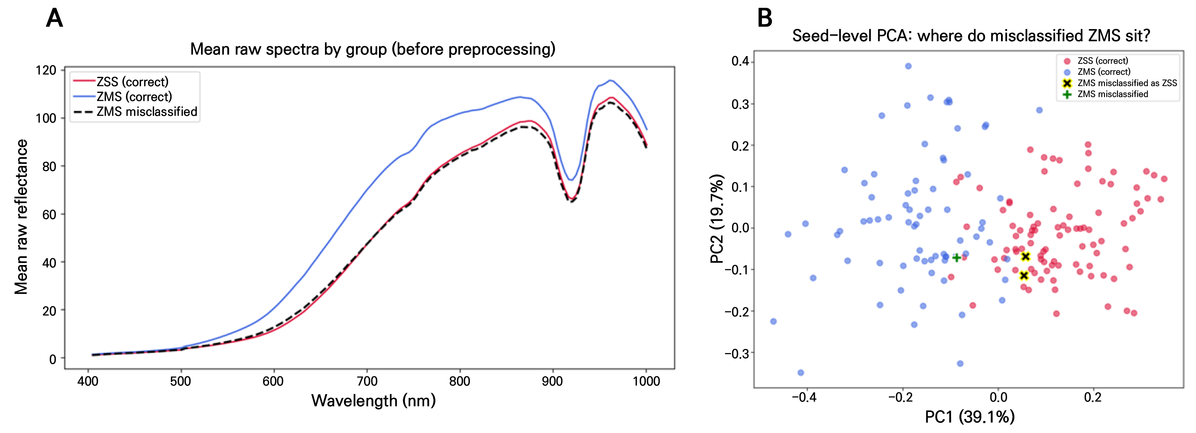
Fig. 8.

Spectral and PCA-based analysis of seed-level misclassifications. (A) Mean raw reflectance spectra of correctly classified ZSS, correctly classified ZMS, and ZMS seeds misclassified as ZSS. (B) Seed-level PCA score plot based on preprocessed spectra, showing the positions of correctly classified and misclassified ZSS and ZMS seeds.

The trained model was subsequently applied to previously unseen hyperspectral images (Fig. 9), and the predicted ZSS and ZMS regions were visualized in red and blue, respectively. During image-level application, adjacent or partially overlapping seeds could be merged into a single contour before majority voting. To address this issue, watershed-based instance segmentation was used to separate individual seeds, after which each segmented seed was classified through majority voting of its pixel-level predictions. Although a small number of locally inconsistent predictions remained, most seeds were assigned to the expected class, and the ZSS seeds were predominantly identified as ZSS and visualized in red. These results demonstrate the potential of the proposed procedure for seed-level classification in hyperspectral images containing multiple adjacent seeds.

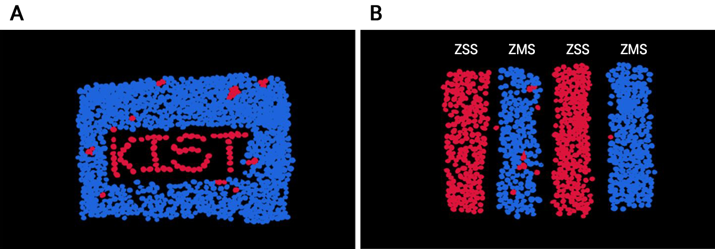
Fig. 9.

Visualization of seed-level classification results obtained from previously unseen hyperspectral images after watershed-based instance segmentation and majority voting. Red and blue indicate seeds classified as ZSS and ZMS, respectively. (A) Seeds were arranged to form the letters “KIST” using ZSS, while the surrounding seeds were ZMS. (B) Four vertically arranged seed groups were placed in the order ZSS, ZMS, ZSS, and ZMS from left to right.

Discussion

This study demonstrated the feasibility of combining hyperspectral imaging (HSI) with AutoGluon to distinguish ZSS from its adulterant, ZMS. The proposed approach provides a non-contact and nondestructive alternative to conventional analytical methods and achieved consistently high classification performance under seed-grouped cross-validation using Savitzky–Golay smoothing, SNV, and first-order derivative preprocessing.

Permutation-based feature importance identified 628.66 nm as the wavelength with the highest mean importance, and the ten most important wavelengths were concentrated in the 596–677 nm region. Because the analysis was performed on SNV- and derivative-preprocessed spectra, these findings are more likely to reflect local spectral-shape and slope variations than raw reflectance intensity alone. Point-biserial correlation analysis also showed relatively high values in the 600–700 nm region. Although the two analyses represent different concepts—univariate association and multivariate model dependence—their agreement supports the relevance of this spectral region to ZSS–ZMS discrimination.

Seed-level misclassification was rare and occurred in both directions, with two ZMS seeds misclassified as ZSS and one ZSS seed misclassified as ZMS among 169 seeds. The two ZMS cases warranted particular attention because they showed lower raw reflectance than typical ZMS and were located near the boundary between the ZSS and ZMS clusters in the preprocessed PCA feature space. They also exhibited lower majority-vote margins than correctly classified seeds. These findings suggest that the remaining errors were associated with spectrally borderline samples rather than being caused solely by brightness differences. Because ZMS-to-ZSS misclassification is particularly important in adulteration detection, future studies should include ZMS samples with a broader range of physical attributes—including color, overall reflectance (luminance), surface characteristics, and seed thickness—as well as greater spectral variability. The use of a confidence threshold or abstention option may also help identify uncertain samples requiring additional inspection.

Several limitations should be acknowledged. All samples were obtained through a single institution, and an independent external validation dataset was not available. In addition, the exclusion of six ZSS and 25 ZMS samples reduced the overall dataset size and increased class imbalance, although balanced accuracy remained close to overall accuracy. Future studies should therefore validate the model using independently collected samples from diverse institutions and market channels, expand the number and diversity of ZMS samples across production lots and harvest years, and further evaluate the robustness of the proposed approach across acquisition sessions, illumination conditions, and instruments.

Despite these limitations, the results demonstrate that HSI combined with AutoGluon has strong potential as a rapid and nondestructive screening tool for the authentication of ZSS and the detection of ZMS adulteration. Given the difficulty of visually distinguishing the two species and the practical risk of adulteration in the herbal medicine market, this study provides an important foundation for the development of more reliable, scalable, and objective quality-control systems.